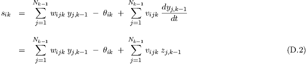
From Eqs. (3.1) and (3.5) we have
|
|
with, for k > 1,
The sik are now directly available without differentiation or integration in the expressions for neuron i in layer k > 1, since the zj,k-1 are “already” obtained through integration in the preceding layer k - 1. The special case k = 1, where differentiation of network input signals is needed to obtain the zj,0, is obtained from a separate numerical differentiation. One may use Eq. (3.16) for this purpose.Eq. (D.1) may also be written as
|
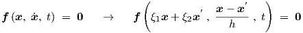
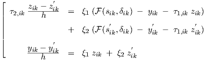
We will apply a discretization according to the scheme
|
where values at previous time points in the discretized expressions are denoted by accents ( ′).
Consequently, a set of implicit nonlinear differential—or differential-algebraic—equations for
variables in the vector x is replaced by a set of implicit nonlinear algebraic equations from
which the unknown new x at a new time point t = t′ + h with h > 0 has to be solved
for a (known) previous x′ at time t′. Different values for the parameters ξ1 and ξ2
allow for the selection of a particular integration scheme. The Forward Euler method
is obtained for ξ1 = 0, ξ2 = 1, the Backward Euler method for ξ1 = 1, ξ2 = 0, the
trapezoidal integration method for ξ1 = ξ2 =  and the second order Adams-Bashforth
method for ξ1 =
and the second order Adams-Bashforth
method for ξ1 =  , ξ2 = -
 [9]. See also [10] for the Backward Euler method. In all
these cases we have ξ2 ≡ 1 - ξ1. In the following, we will exclude the Forward Euler
variant, since it would lead to a number of special cases that require distinct expressions
in order to avoid division by zero, while it also has rather poor numerical stability
properties.
[9]. See also [10] for the Backward Euler method. In all
these cases we have ξ2 ≡ 1 - ξ1. In the following, we will exclude the Forward Euler
variant, since it would lead to a number of special cases that require distinct expressions
in order to avoid division by zero, while it also has rather poor numerical stability
properties.
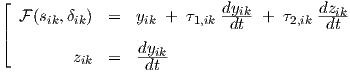
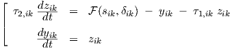
Using Eq. (D.4), we obtain from Eq. (D.3)
|
Provided that ξ1≠0—hence excluding pure Forward Euler—we can solve for yik and zik to obtain the explicit expressions
![⌊ {
2 ′
|| yik = ξ1F(sik,δik) + ξ1ξ2F (sik,δik)
|| [ ] }
|| + - ξ1ξ2 + ξ1τ1,ik- + τ2,ik2- y′ik + ξ1 +-ξ2-τ2,ik z′ik
|| { h h} h
|| 2 τ1,ik τ2,ik
|| ∕ ξ1 + ξ1 h + h2
||
⌈ yik --y′ik ξ2 ′
zik = hξ1 - ξ1 zik](thesis268x.png)
|
where division by zero can never occur for ξ1≠0, h≠0. This equation is a generalization of Eq. (3.4): for ξ1 = 1 and ξ2 = 0, Eq. (D.6) reduces to Eq. (3.4).
The expressions for transient sensitivity are obtained by differentiating Eqs. (D.2) and (D.6) w.r.t. any (scalar) parameter p (indiscriminate whether p resides in this neuron or in a preceding layer), which leads to
![Nk-1 [ ]
∂sik- ∑ dwijk ∂yj,k--1 dθik-
∂p = dp yj,k-1 + wijk ∂p - dp
Nj=k1-1 [ ]
+ ∑ dvijkz + v ∂zj,k--1
j=1 dp j,k- 1 ijk ∂p](thesis269x.png)
|
which is identical to the first equation of (3.8), and
![{
⌊ ∂y [( ) ( ) (∂s )]
| -∂pik = ξ21 ∂∂Fp- + ∂∂sF- -∂ipk
|| [( )′ ik ( )′]
|| ∂F- ( ∂F--)′ ∂sik
|| + ξ1ξ2 ∂p + ∂sik ∂p
|| [ (∂τ1,ik) ( ∂τ2,ik)] ( ′ )
|| - ξ1 --∂p- + 1h- -∂p-- ξ1zik + ξ2zik
|| ( )′
|| + [- ξ ξ + ξ τ1,ik + τ2,ik] ∂yik-
|| 1 2 1 h h2 ∂p
|| [( ) ( )′] }
|| + ξ1-+-ξ2 ∂-τ2,ik z′ik + τ2,ik ∂zik-
|| h ∂p ∂p
|| { }
|| ∕ ξ2 + ξ τ1,ik + τ2,ik
|| 1 1 h h2
||
|| ( ∂y ) (∂y ) ′
|⌈ ∂z ∂pik- - -∂pik ξ ( ∂z )′
-∂ipk = --------hξ--------- - ξ2 -∂ipk
1 1](thesis270x.png)
|
which generalizes the second and third equation of (3.8).
For any integration scheme, the initial partial derivative values are again, as in Eq. (3.9), obtained from the forward propagation of the steady state equations
![⌊
∂s || N∑k-1[ dwijk || ∂yj,k-1|| ] dθik
|| -∂pik|| = -dp--yj,k-1|| + wijk --∂p--|| - dp--
|| |t=0 j=1 |t=0 t=0
|| ∂yik|| = ∂F- + -∂F- ∂sik||
|| ∂p |t=0 ∂p ∂sik ∂p |t=0
|⌈ ||
∂z∂ipk|| = 0
t=0](thesis271x.png)
|
corresponding to dc sensitivity.
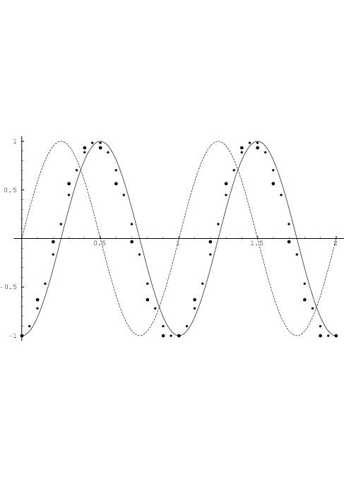
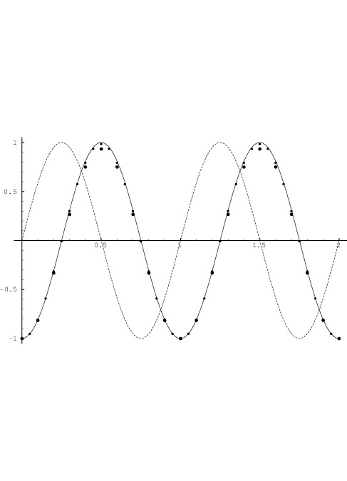
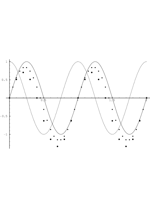
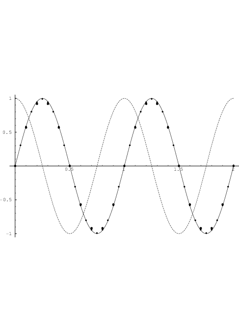
To give an intuitive impression about the accuracy of the Backward Euler method and the trapezoidal integration method for relatively large time steps, it is instructive to consider a concrete example, for instance the numerical time integration of the differential equation ẋ = 2π sin(2πt) with x(0) = -1, to obtain an approximation of the exact solution x(t) = -cos(2πt). Figs. D.1 and D.2 show a few typical results for the Backward Euler method and the trapezoidal integration method, respectively. Similarly, Figs. D.3 and D.4 show results for the numerical time integration of the differential equation ẋ = 2π cos(2πt) with x(0) = 0, to obtain an approximation of the exact solution x(t) = sin(2πt). Clearly, the trapezoidal integration method offers a significantly higher accuracy in these examples. It is also apparent from the results of Backward Euler integration, that the starting point for the integration of a periodic function can have marked qualitative effects on the approximation errors.