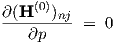
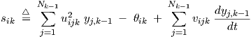
As a special topic, section 3.3 will discuss how monotonicity of the static response of feedforward neural networks can be guaranteed via parameter constraints imposed during learning.
This section first describes numerical techniques for solving the neural differential equations in the time domain. Time domain analysis by means of numerical time integration (and differentiation) is often called transient analysis in the context of circuit simulation. Subsequently, the sensitivity of the solutions for changes in neural network parameters is derived. This then forms the basis for neural network learning by means of gradient-based optimization schemes.
There exist many general algorithms for numerical integration, providing trade-offs between accuracy, time step size, stability and algorithmic complexity. See for instance [9] or [29] for explicit Adams-Bashforth and implicit Adams-Moulton multistep methods. The first-order Adams-Bashforth algorithm is identical to the Forward Euler integration method, while the first-order Adams-Moulton algorithm is identical to the Backward Euler integration method. The second-order Adams-Moulton algorithm is better known as the trapezoidal integration method.
For simplicity of presentation and discussion, and to avoid the intricacies of automatic selection of time step size and integration order1, we will in the main text only consider the use of one of the simplest, but numerically very stable—“A-stable” [29]—methods: the first order Backward Euler method for variable time step size. This method yields algebraic expressions of modest complexity, suitable for a further detailed discussion in this thesis.
In a practical implementation, it may be worthwhile2 to also have the trapezoidal integration method available, since it provides a much higher accuracy for sufficiently small time steps, while this method is also A-stable. Appendix D describes a generalized set of expressions that applies to the Backward Euler method, the trapezoidal integration method and the second order Adams-Bashforth method.
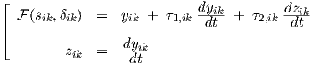
Equation (2.2) for layer k > 0 can be rewritten into two first order differential equations by introducing an auxiliary variable zik as in
|
|
We will apply the Backward Euler integration method to Eq. (3.1), according to the substitution scheme [10]
|
with a local time step h—which may vary in subsequent time steps, allowing for non-equidistant time points—and again denoting values at the previous time point by accents ( ′). This gives the algebraic equations
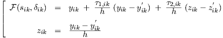
|
Now we have the major advantage that we can, due to the particular form of the differential equations (3.1), explicitly solve Eq. (3.3) for yik and zik to obtain the behaviour as a function of time, and we find for layer k > 0
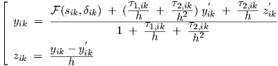
|
for which the sik are obtained from
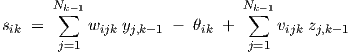
|
where Eq. (3.1) was used to eliminate the time derivative dyj,k-1∕dt from Eq. (2.3). However, for
layer k = 1, the required zj,0 in Eq. (3.5) are not available from the time integration of a neural
differential equation in a preceding layer. Therefore, the zj,0 have to be obtained separately from
a finite difference formula applied to the imposed network inputs yj,0, for example using
zj,0 (yj,0 - yj,0′)∕h, although a more accurate numerical differentiation method may be
preferred3.
(yj,0 - yj,0′)∕h, although a more accurate numerical differentiation method may be
preferred3.
Initial neural states for any numerical integration scheme immediately follow from forward propagation of the explicit equations for the so-called “implicit dc” analysis4, giving the steady state behaviour of one particular neuron i in layer k > 0 at time t = 0
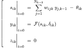
|
by setting all time-derivatives in Eqs. (2.2) and (2.3) to zero. Furthermore,  t=0 = 0 should
be the outcome of the above-mentioned numerical differentiation method in order to keep
Eq. (3.5) consistent with Eq. (3.6).
t=0 = 0 should
be the outcome of the above-mentioned numerical differentiation method in order to keep
Eq. (3.5) consistent with Eq. (3.6).
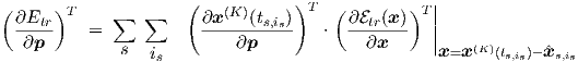
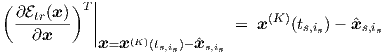
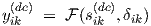
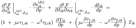
The expressions for transient sensitivity, i.e., partial derivatives w.r.t. parameters, can be obtained by first differentiating Eqs. (3.1) and (3.5) w.r.t. any (scalar) parameter p (indiscriminate whether p resides in this neuron or in a preceding layer), giving
![⌊
∂s Nk∑-1[ dwijk ∂yj,k-1] dθik
|| -∂ipk = -dp--yj,k- 1 + wijk --∂p--- - -dp-
|| j=1
|| N∑k-1[dvijk ∂zj,k-1]
|| + -dp-- zj,k- 1 + vijk--∂p---
|| j=1 ( )
|| ∂F- + -∂F- ∂sik = ∂yik + ∂τ1,ik dyik + τ1,ik -d ∂yik
|| ∂p ∂sik ∂p ∂p ∂p dt ( )dt ∂p
|| ∂τ2,ik dzik -d ∂zik
|| + ∂p dt + τ2,ik dt ∂p
|⌈ ∂z (∂y )
-∂ipk = ddt -∂pik](thesis119x.png)
|
and by subsequently discretizing these differential equations, again using the Backward Euler method. However, a preferred alternative method is to directly differentiate the expressions in Eq. (3.3) w.r.t. any parameter p. The resulting expressions for the two approaches are in this case exactly the same, i.e., independent of the order of differentiation w.r.t. p and discretization w.r.t. t. Nevertheless, in general it is conceptually better to first perform the discretization, and only then the differentiation w.r.t. p. Thereby we ensure that the transient sensitivity expressions will correspond exactly to the discretized time domain behaviour that will later, in section 3.1.3, be used in the minimization of a time domain error measure Etr. A separate approximation, by means of time discretization, of a differential equation and an associated differential equation for its partial derivative w.r.t. p, would not a priori be guaranteed to lead to consistent results for the error measure and its gradient: the time discretization of the partial derivative w.r.t. p of a differential equation need not exactly equal the partial derivative w.r.t. p of the time-discretized differential equation, if only because different discretization schemes might have been applied in the two cases.
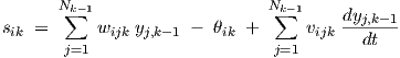
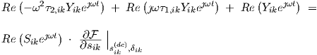
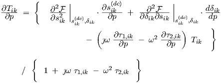
Following the above procedure, the resulting expressions for layer k > 0 are
![⌊
∂s Nk∑-1[ dwijk ∂yj,k-1] dθik
|| -∂ipk = -dp--yj,k- 1 + wijk --∂p--- - -dp-
|| j=1
|| N∑k-1[dvijk ∂zj,k-1]
|| + -dp-- zj,k- 1 + vijk--∂p---
|| j{=1 ( )
|| ∂yik = ∂F- + -∂F- ∂sik - ∂-τ1,ik z
|| ∂p ∂p ∂sik ∂p ∂p ik
|| [ ] ( ) ′ ′
|| + τ1,ik+ τ2,ik2- ∂yik - ∂τ2,ik (zik --zik)-
|| h ( h) ′ }∂p ∂p h
|| τ2,ik- ∂zik
|| + h ∂p
|| { }
|| ∕ 1 + τ1,ik + τ2,ik
|| h h2
|| ( ∂y ) ( ∂y )′
|⌈ -∂ipk - -∂ipk
∂z∂ipk = ---------h---------](thesis120x.png)
|
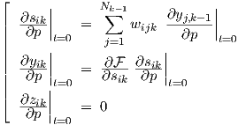
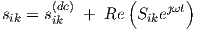
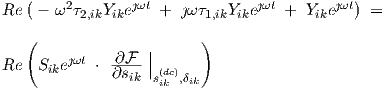
while initial partial derivative values immediately follow from forward propagation of the steady state equations for layer k > 0
![⌊ || N∑k-1[ || || ]
| ∂sik|| = dwijk-yj,k-1|| + wijk ∂yj,k-1|| - dθik
|| ∂p |t=0 j=1 dp |t=0 ∂p t=0 dp
|| ∂yik|| ∂F- -∂F- ∂sik||
|| ∂p |t=0 = ∂p + ∂sik ∂p |t=0
|| |
⌈ ∂zik|| = 0
∂p |t=0](thesis121x.png)
|
corresponding to dc sensitivity. The ∂yj,0∕∂p and ∂zj,0∕∂p, occurring in Eqs. (3.8) and (3.9) for k = 1, are always zero-valued, because the network inputs do not depend on any network parameters.
The partial derivative notation ∂∕∂p was maintained for the parameters τ1,ik and τ2,ik, because they actually represent the bivariate parameter functions τ1(σ1,ik , σ2,ik) and τ2(σ1,ik , σ2,ik), respectively. Particular choices for p must be made to obtain expressions for implementation: if residing in layer k, p is one of the parameters δik, θik, wijk, vijk, σ1,ik and σ2,ik, using the convention that the (neuron input) weight parameters wijk, vijk and the threshold θik belong to layer k, since they are part of the definition of sik in Eq. (2.3).
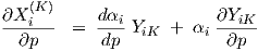
Derivatives needed to calculate the network output gradient via the linear output scaling xi(K) = αi yiK + βi in Eq. (2.5) are given by
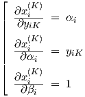
|
where the derivative w.r.t. yiK is used to find network output derivatives w.r.t. network parameters other than αi and βi, since their influence is “hidden” in the time evolution of yiK.
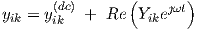
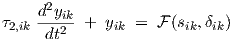
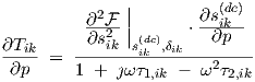
If p resides in a preceding layer, Eq. (3.8) can be simplified, and the partial derivatives can then be recursively found from the expressions
![⌊
Nk∑-1[ ∂y ∂z ]
|| ∂sik = wijk --j,k--1 + vijk---j,k-1
|| ∂p j=1 ∂p ∂p
|| { ( )
|| ∂yik = -∂F- ∂sik
|| ∂p ∂sik ∂p }
|| [τ1,ik τ2,ik] (∂yik) ′ τ2,ik-( ∂zik-)′
|| + h + h2 ∂p + h ∂p
|| { }
|| τ1,ik τ2,ik
|| ∕ 1 + h + h2
|| ( ) ( )′
|⌈ ∂yik - ∂yik
∂zik = ---∂p---------∂p---
∂p h](thesis123x.png)
|
until one “hits” the layer where the parameter resides. The actual evaluation can be done in a feedforward manner to avoid recursion. Initial partial derivative values in this scheme for parameters in preceding layers follow from the dc sensitivity expressions
|
All parameters for a single neuron i in layer k together give rise to a neuron parameter vector p(i,k), here for instance

|
where the τ’s follow from τ1,ik = τ1(σ1,ik , σ2,ik) and τ2,ik = τ2(σ1,ik , σ2,ik). All neuron i
parameter vectors p(i,k) within a particular layer k may be strung together to form a vector p(k),
and these vectors may in turn be joined, also including the components of the network output
scaling vectors α = (α1 , ,αNK )T and β = (β1 ,
 ,βNK )T , to form the network parameter
vector p.
,βNK )T , to form the network parameter
vector p.
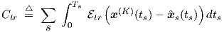
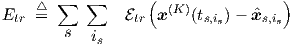
In practice, we may have to deal with more than one time interval (section) with associated time-dependent signals, or waves, such that we may denote the is-th discrete time point in section s by ts,is. (For every starting time ts,1 an implicit dc is performed to initialize a new transient analysis.) Assembling all the results obtained thus far, we can calculate at every time point ts,is the network output vector x(K), and the time-dependent NK-row transient sensitivity derivative matrix Dtr = Dtr(ts,is) for the network output defined by
|
which will be used in gradient-based learning schemes to determine values for all the elements of p. That next step will be covered in section 3.1.3.
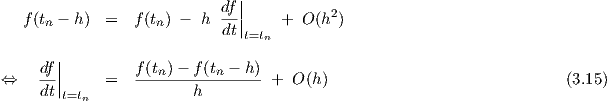
The error5 of the finite difference approximation zj,0 = (yj,0 -yj,0′)∕h for the time derivatives of the neural network inputs, as given in the previous section, is at most proportional to h for sufficiently small h. In other words, the approximation error is O(h), as immediately follows from a Taylor expansion of a function f around a point tn of the (backward) form
However, this approximation error does not accumulate for given network inputs, contrary to the local truncation error in numerical integration.The local truncation error is the integration error made in one time step as a consequence of the discretization of the differential equation. The size of the local truncation error of the Backward Euler integration method is O(h2), but this error accumulates—assuming equidistant time points—to a global truncation error that is also O(h) due to the O(h-1) time steps in a given simulation time interval6. Similarly, the O(h3) local truncation error of the trapezoidal integration method would accumulate to an O(h2) global truncation error, in that case motivating the use of an O(h2) numerical differentiation method at the network input, for example

| (3.16) |
where the right-hand side is the exact time derivative at tn of a parabola interpolating the
points 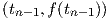 ,
,  and
and  . A Taylor expansion of this expression
then yields
. A Taylor expansion of this expression
then yields
| (3.17) |
for equidistant time points, i.e., for tn+1 - tn = tn - tn-1 = h.
The network inputs at “future” points tn+1 are during neural network learning already available from the pre-determined training data. When these are not available, one may resort to a Backward Differentiation Formula (BDF) to obtain accurate approximations of the time derivative at tn from information at present and past time points [9]. The BDF of order m will give the exact time derivative at tn of an m-th degree polynomial interpolating the network input values at the m + 1 time points tn ,…, tn-m , while causing an error O(hm) in the time derivative of the underlying (generally unknown) real network input function, assuming that the latter is sufficiently smooth—at least Cm+1.
The neural network parameter elements in p have to be determined through some kind of optimization on training data. For the dc behaviour, applied voltages on a device can be used as input to the network, and the corresponding measured or simulated terminal currents as the desired or target output of the network (the target output could in fact be viewed as a special kind of input to the network during learning). For the transient behaviour, complete waves involving (vectors of) these currents and voltages as a function of (discretized) time are needed to describe input and target output. In this thesis, it is assumed that the transient behaviour of the neural network is initialized by an implicit dc analysis at the first time point t = 0 in each section. Large-signal periodic steady state analysis is not considered.
The learning phase of the network consists of trying to model all the specified dc and transient
behaviour as closely as possible, which therefore amounts to an optimization problem. The dc
case can be treated as a special case of transient analysis, namely for time t = 0 only. We can
describe a complete transient training set  ⊔∇ for the network as a collection of tuples. A
number of time sections s can be part of ⊔∇. Each tuple contains the discretized time
ts,is, the network input vector xs,is(0) , and the target output vector
⊔∇ for the network as a collection of tuples. A
number of time sections s can be part of ⊔∇. Each tuple contains the discretized time
ts,is, the network input vector xs,is(0) , and the target output vector  s,is, where the
subscripts s,is refer to the is-th time point in section s. Therefore, ⊔∇ can be written
as
s,is, where the
subscripts s,is refer to the is-th time point in section s. Therefore, ⊔∇ can be written
as
Only one time sample per section ts,is=1 = 0 is used to specify the behaviour for a particular dc
bias condition. The last time point in a section s is called Ts. The target outputs  s,is will
generally be different from the actual network outputs x(K)(ts,is), resulting from network inputs
xs,is(0) at times ts,is . The local time step size h used in the previous sections is simply one of the
ts,is+1 - ts,is .
s,is will
generally be different from the actual network outputs x(K)(ts,is), resulting from network inputs
xs,is(0) at times ts,is . The local time step size h used in the previous sections is simply one of the
ts,is+1 - ts,is .
When dealing with device or subcircuit modelling, behaviour can in
general7
be characterized by (target) currents  (t) flowing for given voltages v(t) as a function of time t.
Here
(t) flowing for given voltages v(t) as a function of time t.
Here  is a vector containing a complete set of independent terminal currents. Due to the
Kirchhoff current law, the number of elements in this vector will be one less than the number of
device terminals. Similarly, v contains a complete set of independent voltages. Their
number is also one less than the number of device terminals, since one can take one
terminal as a reference node (a shared potential offset has no observable physical effect
in classical physics). See also the earlier discussion, and Fig. 2.1, in section 2.1.2.
In such an
is a vector containing a complete set of independent terminal currents. Due to the
Kirchhoff current law, the number of elements in this vector will be one less than the number of
device terminals. Similarly, v contains a complete set of independent voltages. Their
number is also one less than the number of device terminals, since one can take one
terminal as a reference node (a shared potential offset has no observable physical effect
in classical physics). See also the earlier discussion, and Fig. 2.1, in section 2.1.2.
In such an  (v(t)) representation the vectors v and
  would therefore be of equal
length, and the neural network contains identical numbers of inputs (independent
voltages) and outputs (independent currents). The training set would take the form
would therefore be of equal
length, and the neural network contains identical numbers of inputs (independent
voltages) and outputs (independent currents). The training set would take the form

| (3.19) |
and the actual response of the neural network would provide i(v(ts,is)) corresponding to
x(K)(x(0)(ts,is)). Normally one will apply the convention that the j-th element of v refers
to the same device or subcircuit terminal as the j-th element of  or i. Device or
subcircuit parameters for specifying geometry or temperature can be incorporated
by assigning additional neural network inputs to these parameters, as is shown in
Appendix B.
or i. Device or
subcircuit parameters for specifying geometry or temperature can be incorporated
by assigning additional neural network inputs to these parameters, as is shown in
Appendix B.
Returning to our original general notation of Eq. (3.18), we now define a time domain error measure Etr for accumulating the errors implied by the differences between actual and target outputs over all network outputs (represented by a difference vector), over all time points indexed by is , and over all sections s,
where the error function  tr(⋅) is a function having a single, hence global, minimum at the point
where its vector argument is zero-valued. Usually one will for semantical reasons prefer a
function that fulfills tr(0) = 0, although this is not strictly necessary.
tr(⋅) is a function having a single, hence global, minimum at the point
where its vector argument is zero-valued. Usually one will for semantical reasons prefer a
function that fulfills tr(0) = 0, although this is not strictly necessary.
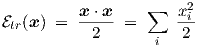
Etr is just the discrete-time version of the continuous-time cost function Ctr, often encountered in the literature:
| (3.21) |
However, target waves of physical systems can in practice rarely be specified by continuous functions (even though their behaviour is continuous, one simply doesn’t know the formula’s that capture that behaviour), let alone that the integration could be performed analytically. Therefore, Etr is much more practical than Ctr.
In the literature on optimization, the scalar function tr of a vector argument is often simply
half the sum of squares of the elements, or in terms of the inner product
| (3.22) |
which fulfills tr(0) = 0.
In order to deal with small (exponentially decreasing or increasing) device currents, still
other modelling-specific definitions for tr may be used, based on a generalized form
tr . These modelling-specific forms for tr will not be covered in this
thesis.
. These modelling-specific forms for tr will not be covered in this
thesis.
Some of the most efficient optimization schemes employ gradient information—partial derivatives of an error function w.r.t. parameters—to speed up the search for a minimum of a differentiable error function. The simplest—and also one of the poorest—of those schemes is the popular steepest descent method8. Many variations on this theme exist, like the addition of a momentum term, or line searches in a particular descent direction.
In the following, the use of steepest descent is described as a simple example case to illustrate the principles of optimization, but its use is definitely not recommended, due to its generally poor performance and its non-guaranteed convergence for a given learning rate. An important aspect of the basic methods described in this thesis is that any general optimization scheme can be used on top of the sensitivity calculations9. There exists a vast literature on optimization convergence properties, so we need not separately consider that problem within our context. Any optimization scheme that is known to be convergent will also be convergent in our neural network application.
Steepest descent is the basis of the popular error backpropagation method, and many people still use it to train static feedforward neural networks. The motivation for its use could be, apart from simplicity, that backpropagation with steepest descent can easily be written as a set of local rules, where each neuron only needs biasing information entering in a forward pass through its input weights and error sensitivity information entering in a backward pass through its output. However, for a software implementation on a sequential computer, the strict locality of rules is entirely irrelevant, and even on a parallel computer system one could with most optimization schemes still apply vectorization and array processing to get major speed improvements.
Steepest descent would imply that the update vector for the network parameters is calculated from
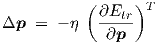
| (3.23) |
where η > 0 is called the learning rate. A so-called momentum term can simply be added to Eq. (3.23) by using
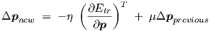
| (3.24) |
where μ ≥ 0 is a parameter controlling the persistence with which the learning scheme proceeds in a previously used parameter update direction. Typical values for η and μ used in small static backpropagation neural networks with the logistic activation function are η = 0.5 and μ = 0.9, respectively. Unfortunately, the steepest descent scheme is not scaling-invariant, so proper values for η and μ may strongly depend on the problem at hand. This often results in either extremely slow convergence or in wild non-convergent parameter oscillations. The fact that we use the gradient w.r.t. parameters of a set of differential equations with dynamic (electrical) variables in a system with internal state variables implies that we actually perform transient sensitivity in terms of circuit simulation theory.
With (3.20), we find that
| (3.25) |
The first factor has been obtained in the previous sections as the time-dependent transient
sensitivity matrix Dtr = Dtr(ts,is). For tr defined in Eq. (3.22), the second factor in Eq. (3.25)
would become
| (3.26) |
In this section we consider the small-signal response of dynamic feedforward neural networks in the frequency domain. The sensitivity of the frequency domain response for changes in neural network parameters is derived. As in section 3.1 on time domain learning, this forms the basis for neural network learning by means of gradient-based optimization schemes. However, here we are dealing with learning in a frequency domain representation. Frequency domain learning can be combined with time domain learning.
We conclude with a few remarks on the modelling of bias-dependent cut-off frequencies and on the generality of a combined static (dc) and small-signal frequency domain characterization of behaviour.
Devices and subcircuits are often characterized in the frequency domain. Therefore, it may prove worthwhile to provide facilities for optimizing for frequency domain data as well. This is merely a matter of convenience and conciseness of representation, since a time domain representation is already completely general.
Conventional small-signal ac analysis techniques neglect the distortion effects due to circuit nonlinearities. This means that under a single-frequency excitation, the circuit is supposed to respond only with that same frequency. However, that assumption in general only holds for linear(ized) circuits, for which responses for multiple frequencies then simply follow from a linear superposition of results obtained for single frequencies.
The linearization of a nonlinear circuit will only yield the same behaviour as the original circuit if the signals involved are vanishingly small. If not, the superposition principle no longer holds. With input signals of nonvanishing amplitude, even a single input frequency will normally generate more than one frequency in the circuit response: higher harmonics of the input signal arise, with frequencies that are integer multiples of the input frequency. Even subharmonics can occur, for example in a digital divider circuit. If a nonlinear circuit receives signals involving multiple input frequencies, then in principle all integer-weighted combinations of these input frequencies will appear in the circuit response.
A full characterization in the frequency domain of nonlinear circuits is possible when the (steady state) circuit response is periodic, since the Fourier transformation is known to be bijective.
On the other hand, in modelling applications, even under a single-frequency excitation, and with a periodic circuit response, the storage and handling of a large—in principle infinite—number of harmonics quickly becomes prohibitive. The typical user of neural modelling software is also not likely to be able to supply all the data for a general frequency domain characterization.
Therefore, a parameter sensitivity facility for a bias-dependent small-signal ac analysis is probably the best compromise, by extending the general time domain characterization, which does include distortion effects, with the concise small-signal frequency domain characterization: thus we need (small-signal) ac sensitivity in the optimization procedures in addition to the transient sensitivity that was discussed before.
Small-signal ac analysis is often just called ac analysis for short.
The small-signal ac analysis and the corresponding ac sensitivity for gradient calculations will now be described for the feedforward dynamic neural networks as defined in the previous sections. First we return to the single-neuron differential equations (2.2) and (2.3), which are repeated here for convenience:

| (3.27) |
| (3.28) |
The time-dependent part of the signals through the neurons is supposed to be (vanishingly) small, and is represented as the sum of a constant (dc) term and a (co)sinusoidal oscillation
| (3.29) |
| (3.30) |
with frequency ω and time t, and small magnitudes |Sik|, |Y ik| ; the phasors Sik and Y ik are complex-valued. (The capitalized notation Y ik should not be confused with the admittance matrix that is often used in the physical or electrical modelling of devices and subcircuits.) Substitution of Eqs. (3.29) and (3.30) in Eq. (3.27), linearizing the nonlinear function around the dc solution, hence neglecting any higher order terms, and then eliminating the dc offsets using the dc solution
| (3.31) |
yields
|
Since Re(a) + Re(b) = Re(a + b) for any complex a and b , and also λRe(a) = Re(λa) for any real λ, we obtain
|
This equation must hold at all times t. For example, substituting t = 0 and t =  (making use
of the fact that Re(ȷa) = -Im(a) for any complex a), and afterwards combining the two
resulting equations into one complex equation, we obtain the neuron ac equation
(making use
of the fact that Re(ȷa) = -Im(a) for any complex a), and afterwards combining the two
resulting equations into one complex equation, we obtain the neuron ac equation

|
We can define the single-neuron transfer function
which characterizes the complex-valued ac small-signal response of an individual neuron to its own net input. This should not be confused with the elements of the transfer matrices H(k), as defined further on. The elements of H(k) will characterize the output response of a neuron in layer k w.r.t. to a particular network input. Tik is therefore a “local” transfer function. It should also be noted, that Tik could become infinite. For instance with τ1,ik = 0 and ω2τ2,ik = 1. This situation corresponds to the time domain differential equation
| (3.36) |
from which one finds that substitution of yik = c + acos(ωt), with real-valued constants a and c,
and ω2τ2,ik = 1, yields  (sik,δik) = c, such that the time-varying part of sik must be zero (or
vanishingly small); but then the ratio of the time-varying parts of yik and sik must be infinite, as
was implied by the transfer function Tik. The oscillatory behaviour in yik has become
self-sustaining, i.e., we have resonance. This possibility can be excluded by using appropriate
parameter functions τ1,ik = τ1(σ1,ik , σ2,ik) and τ2,ik = τ2(σ1,ik , σ2,ik). As long as τ1,ik≠0, we
have a term that prevents division by zero through an imaginary part in the denominator of
Tik .
(sik,δik) = c, such that the time-varying part of sik must be zero (or
vanishingly small); but then the ratio of the time-varying parts of yik and sik must be infinite, as
was implied by the transfer function Tik. The oscillatory behaviour in yik has become
self-sustaining, i.e., we have resonance. This possibility can be excluded by using appropriate
parameter functions τ1,ik = τ1(σ1,ik , σ2,ik) and τ2,ik = τ2(σ1,ik , σ2,ik). As long as τ1,ik≠0, we
have a term that prevents division by zero through an imaginary part in the denominator of
Tik .
The ac relations describing the connections to preceding layers will now be considered, and will largely be presented in scalar form to keep their correspondence to the feedforward network topology more visible. This is often useful, also in a software implementation, to keep track of how individual neurons contribute to the overall neural network behaviour. For layer k > 1, we obtain from Eq. (3.28)
| (3.37) |
since the θik only affect the dc part of the behaviour. Similarly, from Eq. (2.4), for the neuron layer k = 1 connected to the network input
| (3.38) |
with phasor Xj(0) the complex j-th ac source amplitude at the network input, as in
| (3.39) |
which in input vector notation obviously takes the form
| (3.40) |
The output of neurons in the output layer is of the form
| (3.41) |
At the output of the network, we obtain from Eq. (2.5) the linear phasor scaling transformation
| (3.42) |
since the βi only affect the dc part of the behaviour. The network output can also be written in the form
| (3.43) |
with its associated vector notation
| (3.44) |
The small-signal response of the network to small-signal inputs can for a given bias and frequency be characterized by a network transfer matrix H. The elements of this complex matrix are related to the elements of the transfer matrix H(K) for neurons i in the output layer via
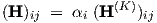
| (3.45) |
When viewed on the network scale, the matrix H relates the network input phasor vector X(0) to the network output phasor vector X(K) through
| (3.46) |
The complex matrix element (H)ij can be obtained from a device or subcircuit by observing the i-th output while keeping all but the j-th input constant. In that case we have (H)ij = Xi(K)∕Xj(0), i.e., the complex matrix element equals the ratio of the i-th output phasor and the j-th input phasor.
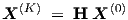
Transfer matrix relations among subsequent layers are given by
| (3.47) |
where j still refers to one of the network inputs, and k = 1, ,K can be used if we define a
(dummy) network input transfer matrix via Kronecker delta’s as
,K can be used if we define a
(dummy) network input transfer matrix via Kronecker delta’s as
| (3.48) |
The latter definition merely expresses how a network input depends on each of the network inputs, and is introduced only to extend the use of Eq. (3.47) to k = 1. In Eq. (3.47), two transfer stages can be distinguished: the weighted sum, without the Tik factor, represents the transfer from outputs of neurons n in the preceding layer k - 1 to the net input Sik, while Tik represents the transfer factor from Sik to Y ik through the single neuron i in layer k.
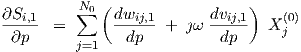
For learning or optimization purposes, we will need the partial derivatives of the ac neural network response w.r.t. parameters, i.e., ac sensitivity. From Eqs. (3.34) and (3.35) we have
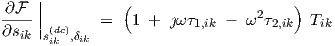
| (3.49) |
and differentiation w.r.t. any parameter p gives for any particular neuron
|
from which  can be obtained as
|
Quite analogous to the transient sensitivity analysis section, it is here still indiscriminate whether p resides in this particular neuron (layer k, neuron i) or in a preceding layer. Also, particular choices for p must be made to obtain explicit expressions for implementation: if residing in layer k, p is one of the parameters δik, θik, wijk, vijk, σ1,ik and σ2,ik, using the convention that the (neuron input) weight parameters wijk, vijk, and threshold θik belong to layer k, since they are part of the definition of sik in Eq. (3.28). Therefore, if p resides in a preceding layer, Eq. (3.51) simplifies to
|
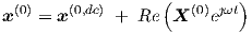
The ac sensitivity treatment of connections to preceding layers runs as follows. For layer k > 1, we obtain from Eq. (3.37)
![∂Sik N∑k-1[( dwijk dvijk) ∂Yj,k- 1]
-----= ----- + ȷω ----- Yj,k-1 + (wijk + ȷω vijk) -------
∂p j=1 dp dp ∂p](thesis181x.png)
|
and similarly, from Eq. (3.38), for the neuron layer k = 1 connected to the network input
|
since Xj(0) is an independent complex j-th ac source amplitude at the network input.
For the output of the network, we obtain from Eq. (3.42)
|
In terms of transfer matrices, we obtain from Eq. (3.45), by differentiating w.r.t. p
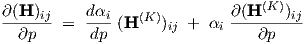
|
and from Eq. (3.47)
for k = 1, ,K, with
| (3.58) |
from differentiation of Eq. (3.48). It is worth noting, that for parameters p residing in the preceding (k - 1)-th layer, ∂(H(k-1))nj∕∂p will be nonzero only if p belongs to the n-th neuron in that layer. However, ∂Tik∕∂p is generally nonzero for any parameter of any neuron in the (k - 1)-th layer that affects the dc solution, from the second derivatives w.r.t. s in Eq. (3.50).
We can describe an ac training set ⊣⌋ for the network as a collection of tuples. Transfer matrix
“curves” can be specified as a function of frequency f (with ω = 2πf) for a number of dc bias
conditions b characterized by network inputs xb(0). Each tuple of ⊣⌋ contains for some bias
condition b an ib-th discrete frequency fb,ib, and for that frequency the target transfer
matrix10
 b,ib, where the subscripts b,ib refer to the ib-th frequency point for bias condition b. Therefore,
⊣⌋ can be written as
b,ib, where the subscripts b,ib refer to the ib-th frequency point for bias condition b. Therefore,
⊣⌋ can be written as
Analogous to the treatment of transient sensitivity, we will define a 3-dimensional ac sensitivity tensor Dac, which depends on dc bias and on frequency. Assembling all network parameters into a single vector p, one may write
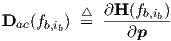
| (3.60) |
which will be used in optimization schemes. Each of the complex-valued sensitivity
tensors Dac(fb,ib) can be viewed as (sliced into) a sequence of derivative matrices,
each derivative matrix consisting of the derivative of the transfer matrix H w.r.t. one
particular (scalar) parameter p. The elements  of these matrices follow from
Eq. (3.56).
of these matrices follow from
Eq. (3.56).
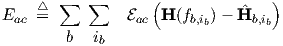
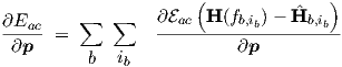
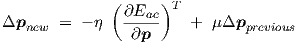
We still must define an error function for ac, thereby enabling the use of gradient-based optimization schemes like steepest descent, or the Fletcher-Reeves and Polak-Ribiere conjugate gradient optimization methods [16]. If we follow the same lines of thought and similar notations as used in section 3.1.3, we may define a frequency domain error measure Eac for accumulating the errors implied by the differences between actual and target transfer matrix (represented by a difference matrix), over all frequencies indexed by ib and over all bias conditions b (for which the network was linearized). This gives
By analogy with tr in Eq. (3.22), we could choose a sum-of-squares form, now extended to
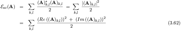
complex matrices A via
ac. The derivative of ac
w.r.t. the real-valued parameter vector p is given by
![∑ [ ( ) ( ) ]
∂Eac(A-)-= Re ((A)k,l) Re ∂-(A-)k,l + Im ((A )k,l) Im ∂-(A-)k,l
∂p k,l ∂p ∂p](thesis195x.png)
| (3.63) |
With A = H(fb,ib) - b,ib we see that the
  =
=  are the elements of the bias
and frequency dependent ac sensitivity tensor Dac = Dac(fb,ib) obtained in Eq. (3.60). So
Eqs. (3.62) and (3.63) can be evaluated from the earlier expressions.
are the elements of the bias
and frequency dependent ac sensitivity tensor Dac = Dac(fb,ib) obtained in Eq. (3.60). So
Eqs. (3.62) and (3.63) can be evaluated from the earlier expressions.
For Eac in Eq. (3.61) we simply have
| (3.64) |
Once we have defined scalar functions ac and Eac, we may apply any general gradient-based
optimization scheme on top of the available data. To illustrate the similarity with the
earlier treatment of time domain neural network learning, we can immediately write
down the expression for ac-optimization by steepest descent with a momentum term
| (3.65) |
Of course, one can easily combine time domain optimization with frequency domain optimization, for instance by minimizing λ1Etr + λ2Eac through
![[ ( )T ( )T ]
Δp = - η λ ∂Etr- + λ ∂Eac- + μ Δp
new 1 ∂p 2 ∂p previous](thesis201x.png)
| (3.66) |
where λ1 and λ2 are constants for arbitrarily setting the relative weights of time domain
and frequency domain optimization. Their values may be set during a pre-processing
phase applied to the time domain and frequency domain target data. An associated
training set is constructed by the union of the sets in Eqs. (3.18) and (3.59) as in
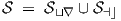
| (3.67) |
The transient analysis and small-signal ac analysis are based upon exactly the same set of neural network differential equations. This makes the transient analysis and small-signal ac analysis mutually consistent to the extent to which we may neglect the time domain errors caused by the approximative numerical differentiation of network input signals and the accumulating local truncation errors due to the approximative numerical integration methods. However, w.r.t. time domain optimization and frequency domain optimization, we usually have cost functions and target data that are defined independently for both domains, such that a minimum of the time domain cost function Etr need not coincide with a minimum of the frequency domain cost function Eac, even if transient analysis and small-signal ac analysis are performed without introducing numerical errors.
As an illustration of the frequency domain behaviour of a neural network, we will calculate and
plot the transfer matrix for the simplest possible network, a 1-1 network consisting of just a
single neuron with a single input. Using a linear function (sik) = sik, which could also be
viewed as the linearized behaviour of a nonlinear (sik), we find that the 1 × 1 “matrix” H(K) is
given by
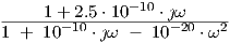
| (3.68) |
This expression for H(K) is obtained from the application of Eqs. (3.35), (3.45), (3.47) and (3.48). For this very simple example, one could alternatively obtain the expression for H(K) “by inspection” directly from Eqs. (2.2), (2.4) and (2.5).
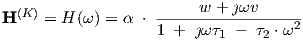
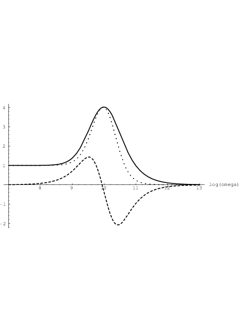
We may set the parameters for an overdamped neuron, as discussed in section 2.3.1, with Q = 0.4 and ω0 = 1010 rad/s, such that τ1 = 1∕(ω0Q) = 2.5 ⋅ 10-10s and τ2 = 1∕ω02 = 10-20s2, and use α = 1, w = 1, and v = 10-9. Fig. 3.1 shows the complex-valued transfer H(ω) for this choice of parameters in a 3-dimensional parametric plot. Also shown are the projections of the real and imaginary parts of H(ω) onto the sides of the surrounding box. Fig. 3.2 shows the real and imaginary parts of H(ω), as well as the magnitude |H(ω)|.
 .
.
 (dotted), Im
 (dashed), and |H(ω)| (solid).
It is clear from these figures that H(ω) has a vanishing imaginary part for very low frequencies, while the transfer magnitude |H(ω)| vanishes for very high frequencies due to the nonzero τ2. |H(ω)| here peaks11 in the neighbourhood of ω0. The fact that at low frequencies the imaginary part increases with frequency is typical for quasistatic models of 2-terminal devices. However, with quasistatic models the imaginary part would keep increasing up to infinite frequencies, which would be unrealistic.
Another important observation is that for a single neuron the eigenvalues, and hence the eigenfrequencies and cut-off frequencies, are bias-independent. In general, a device or subcircuit may have small-signal eigenfrequencies that are bias dependent.
Nevertheless, a network constructed of neurons as described by Eqs. (2.2) and (2.3) can still
overcome this apparent limitation, because the transfer of signals to the network output is bias
dependent: the derivative w.r.t. sik of the neuron input nonlinearity 2 varies, with bias, within
the range [0,1]. The small-signal transfer through the neuron can therefore be controlled by the
input bias sik. By gradually switching neurons with different eigenfrequencies on or off through
the nonlinearity, one can still approximate the behaviour of a device or subcircuit with
bias-dependent eigenfrequencies. For instance, in modelling the bias-dependent cut-off
frequency of bipolar transistors, which varies typically by a factor of about two within the
relevant range of controlling collector currents, one can get very similar shifts in the
effective cut-off frequency by calculating a bias-weighted combination of two (or more)
bias-independent frequency transfer curves, having different, but constant, cut-off
frequencies. This approach works as long as the range in cut-off frequencies is not too
large; e.g., with the cut-off frequencies differing by no more than a factor of about two
in a bias-weighted combination of two bias-independent frequency transfer curves.
Otherwise, a kind of step (intermediate level) is observed in the frequency transfer
curves12.
As a concrete illustration of this point, one may consider the similarity of the transfer curves
![H (ω,x) = ------[--1--------]
1 1 + ȷω x--+ 1--x-
ω2 ω1](thesis209x.png)
| (3.69) |
which represents an x-bias dependent first order cut-off frequency, and
| (3.70) |
in which two curves with constant cut-off frequencies are weighted by bias-dependent factors. In
a log-log plot, with x in [0,1], and ω2∕ω1 = 2, this gives results like those shown in Fig. 3.3, for
x ∈{0, ,
, ,
, ,1}. The continuous curves for
  are similar to the dashed curves for
  . A
better match can, when needed, be obtained by a more complicated weighting of transfer curves.
. A
better match can, when needed, be obtained by a more complicated weighting of transfer curves.
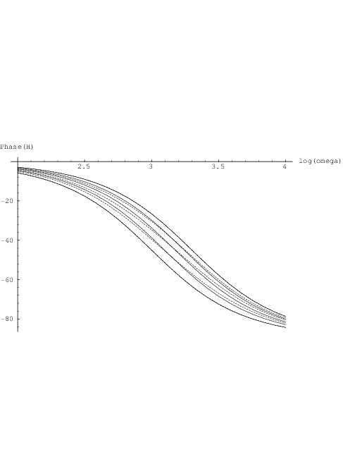
 H1(log ω,x) (continuous) and
  H2(log ω,x) (dashed), in degrees.
Results for the phase shift, shown in Fig. 3.4, are also rather similar for both cases. Consequently, there is still no real need to make τ1,ik and/or τ2,ik dependent on sik, which would otherwise increase the computational complexity of the sensitivity calculations. However, it is worthwhile to note that the left-hand side of Eq. (2.2) would even then give a linear homogeneous differential equation in yik, so we could still use the analytic results obtained in section 2.3.1 with the parameters τ1,ik and τ2,ik replaced by functions τ1,ik(sik) and τ2,ik(sik), respectively. If parameter functions τ1(σ1,ik , σ2,ik) and τ2(σ1,ik , σ2,ik) were used, the same would apply with the parameters σ1,ik and σ2,ik replaced by functions σ1,ik(sik) and σ2,ik(sik), respectively.
The question could be raised, how general a small-signal frequency domain characterization can be, in combination with dc data, when compared to a large-signal time domain characterization. This is a fundamental issue, relating to the kind of data that is needed to fully characterize a device or subcircuit, indiscriminate of any limitations in a subsequently applied modelling scheme, and indiscriminate of limitations in the amount of data that can be acquired in practice.
One could argue, that in a combined ac/dc characterization, the multiple bias points used in determining the dc behaviour and in setting the linearization points for small-signal ac behaviour, together provide the generality to capture both nonlinear and dynamic effects. If the number of bias points and the number of frequency points were sufficiently large, one might expect that the full behaviour of any device or subcircuit can be represented up to arbitrary accuracy. The multiple bias conditions would then account for the nonlinear effects, while the multiple frequencies would account for the dynamic effects.
Intuitively appealing as this argument may seem, it is not valid. This is most easily seen by means of a counterexample. For this purpose, we will once again consider the peak detector circuit that was discussed for other reasons in section 2.6. The circuit consists of a linear capacitor in series with a purely resistive diode, the latter acting as a nonlinear resistor with a monotonic current-voltage characteristic. The voltage on the shared node between diode and capacitor follows the one-sided peaks in a voltage source across the series connection. The diode in this case represents the nonlinearity of the circuit, while the series connection of a capacitor and a (nonlinear) resistor will lead to a non-quasistatic response. However, when performing dc and (small-signal) ac analyses, or dc and ac measurements, the steady state operating point will always be the one with the full applied voltage across the capacitor, and a zero voltage across the diode. This is because the dc current through a capacitor is zero, while this current is “supplied” by the diode which has zero current only at zero bias. Consequently, whatever dc bias is applied to the circuit, the dc and ac behaviour will remain exactly the same, being completely insensitive to the overall shape of the monotonic nonlinear diode characteristic—only the slope of the current-voltage characteristic at (and through) the origin plays a role. Obviously, the overall shape of the nonlinear diode characteristic would affect the large-signal time domain behaviour of the peak detector circuit.
Apparently, we here have an example in which one can supply any amount of dc and (small-signal) ac data without capturing the full behaviour exhibited by the circuit with signals of nonvanishing amplitude in the time domain.
This section shows how feedforward neural networks can be guaranteed to preserve monotonicity in their multidimensional static behaviour, by imposing constraints upon the values of some of the neural network parameters.
The multidimensional dc current characteristics of devices like MOSFETs and bipolar transistors are often monotonic in an appropriately selected voltage coordinate system13. Preservation of monotonicity in the CAD models for these devices is very important to avoid creating additional spurious circuit solutions to the equations obtained from the Kirchhoff current law. However, transistor characteristics are typically also very nonlinear, at least in some of their operating regions, and it turns out to be extremely hard to obtain a model that is both accurate, smooth, and monotonic.
Table modelling schemes using tensor products of B-splines do guarantee monotonicity preservation when using a set of monotonic B-spline coefficients [11, 39], but they cannot accurately describe—with acceptable storage efficiency—the highly nonlinear parts of multidimensional characteristics. Other table modelling schemes allow for accurate modelling of highly nonlinear characteristics, often preserving monotonicity, but generally not guaranteeing it. In [39], two such schemes were presented, but guarantees for monotonicity preservation could only be provided when simultaneously giving up on the capability to efficiently model highly nonlinear characteristics.
In this thesis, we have developed a neural network approach that allows for highly nonlinear
modelling, due to the choice of in Eq. (2.6), Eq. (2.7) or Eq. (2.16), while giving infinitely
smooth results—in the sense of being infinitely differentiable. Now one could ask whether it is
possible to include guarantees for monotonicity preservation without giving up the nonlinearity
and smoothness properties. We will show that this is indeed possible, at least to a certain
extent14.
Recalling that each of the in Eqs. (2.6), (2.7) and (2.16) is already known to be
monotonically increasing in its non-constant argument sik, we will address the necessary
constraints on the parameters of sik, as defined in Eq. (2.3), given only the fact that is
monotonically increasing in sik. To this purpose, we make use of the knowledge that the sum of
two or more (strictly) monotonically increasing (decreasing) 1-dimensional functions is also
(strictly) monotonically increasing (decreasing). This does generally not apply to the difference
of such functions.
Throughout a feedforward neural network, the weights intermix the contributions of the network inputs. Each of the network inputs contributes to all outputs of neurons in the first hidden layer k = 1. Each of these outputs in turn contributes to all outputs of neurons in the second hidden layer k = 2, etc. The consequence is, that any given network input contributes to any particular neuron through all weights directly associated with that neuron, but also through all weights of all neurons in preceding layers.
In order to guarantee network dc monotonicity, the number of sign changes by dc weights wijk must be the same through all paths from any one network input to any one network output15. This implies that between hidden (non-input, non-output) layers, all interconnecting wijk must have the same sign. For the output layer one can afford the freedom to have the same sign for all wij,K connecting to one output neuron, while this sign may differ for different output neurons. However, this does not provide any advantage, since the same flexibility is already provided by the output scaling in Eq. (2.5): the sign of αi can set (switch) the monotonicity “orientation” (i.e., increasing or decreasing) independently for each network output. The same kind of sign freedom—same sign for one neuron, but different signs for different neurons—is allowed for the wij,1 connecting the network inputs to layer k = 1. Here the choice makes a real difference, because there is no additional linear scaling of network inputs like there is with network outputs. However, it is hard to decide upon appropriate signs through continuous optimization, because it concerns a discrete choice. Therefore, the following algorithm will allow the use of optimization for positive wijk only, by a simple pre- and postprocessing of the target data. The algorithm involves four main steps:
Optionally verify that the target output of the selected neuron is indeed monotonic with each of the network inputs, according to the user-specified, or data-derived, monotonicity orientation. The target data for the other network outputs should—up to a collective sign change for each individual output—have the same monotonicity orientation.
| (3.71) |
replacing Eq. (2.3). The sensitivity equations derived before need to be modified correspondingly, but the details of that procedure are omitted here.
The choice made in the first step severely restricts the possible monotonicity orientations for the other network outputs: they have either exactly the same orientation (if their αj have the same sign as the αi of the selected output neuron), or exactly the reverse (for αj of opposite sign). This means, for example, that if the selected output is monotonically increasing as a function of two inputs, it will be impossible to have another output which increases with one input and decreases with the other: that output will either have to increase or to decrease with both inputs.
If this is a problem, one can resort to using different networks to separately model the incompatible outputs. However, in transistor modelling this problem may often be avoided, because these are gated devices with a main current entering one device terminal, and with the approximate reverse current entering another terminal to obey the Kirchhoff current law. The small current of the controlling terminal will generally not affect the monotonicity orientation of any of the main currents, and need also not be modelled because modelling the two main currents suffices (again due to the Kirchhoff law), at least for a 3-terminal device. One example is the MOSFET, where the drain current Id increases with voltages V gs and V gd, while the source current Is decreases with these voltages. Another example is the bipolar transistor, where the collector current Ic increases with voltages V be and V bc, while the emitter current Ie decreases with these voltages17.


![(k) N∑k-1
∂(H---)ij = ∂Tik (wink + ȷωvink) (H (k- 1))nj
∂p ∂p n=1
Nk∑-1[ ( )
+ Tik dwink-+ ȷωdvink (H (k-1))nj
n=1 dp dp
]
∂ (H (k-1))nj
+ (wink + ȷωvink)----∂p---- (3.57)](thesis185x.png)