A practical introduction to the methods described in this section can be found in [17], as well as in many other books, so we will only add a few notes.
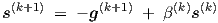
The simplest gradient-based optimization scheme is the steepest descent method. In the present software implementation more efficient methods are provided, among which the Fletcher-Reeves and Polak-Ribiere conjugate gradient optimization methods [16]. Its detailed discussion, especially w.r.t. 1-dimensional search, would lead too far beyond the presentation of basic modelling principles, and would in fact require a rather extensive introduction to general gradient-based optimization theory. However, a few remarks on the algorithmic part may be useful to give an idea about the structure and (lack of) complexity of the method. Basically, conjugate gradient defines subsequent search directions s by
|
| (A.1) |
where the superscript indicates the iteration count. Here g is the gradient of an error or cost
function E which has to be minimized by choosing suitable parameters p; g = ∇E, or in terms
of notations that we used before, g =  T . If β(k) = 0 ∀k, this scheme corresponds to
steepest descent with learning rate η = 1 and momentum μ = 0, see Eq. (3.24). However, with
conjugate gradient, generally only β(0) = 0 and with the Fletcher-Reeves scheme, for k = 1,2,…,
T . If β(k) = 0 ∀k, this scheme corresponds to
steepest descent with learning rate η = 1 and momentum μ = 0, see Eq. (3.24). However, with
conjugate gradient, generally only β(0) = 0 and with the Fletcher-Reeves scheme, for k = 1,2,…,
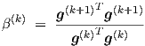
| (A.2) |
while the Polak-Ribiere scheme involves
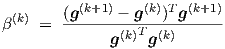
| (A.3) |
For quadratic functions E these two schemes for β(k) can be shown to be equivalent, which
implies that the schemes will for any nonlinear function E behave similarly near a
smooth minimum, due to the nearly quadratic shape of the local Taylor expansion. New
parameter vectors p are obtained by searching for a minimum of E in the s direction by
calculating the value of the scalar parameter α which minimizes E(p(k) + α s(k)). The new
point in parameter space thus obtained becomes the starting point p(k+1) for the next
iteration, i.e., the next 1-dimensional search. The details of 1-dimensional search are
omitted here, but it typically involves estimating the position of the minimum of E
(only in the search direction!) through interpolation of subsequent points in each
1-dimensional search by a parabola or a cubic polynomial, of which the minima can
be found analytically. The slope along the search direction is given by  = sT g.
Special measures have to be taken to ensure that E will never increase with subsequent
iterations.
= sT g.
Special measures have to be taken to ensure that E will never increase with subsequent
iterations.
The background of the conjugate gradient method lies in a Gram-Schmidt orthogonalization procedure, which simplifies to the Fletcher-Reeves scheme for quadratic functions. For quadratic functions, the optimization is guaranteed to reach the minimum within a finite number of exact 1-dimensional searches: at most n, where n is the number of parameters in E. For more general forms of E, no such guarantees can be given, and a significant amount of heuristic knowledge is needed to obtain an implementation that is numerically robust and that has good convergence properties. Unfortunately, this is still a bit of an art, if not alchemy.
Finally, it should be noted that still more powerful optimization methods are known. Among them, the so-called BFGS quasi-Newton method has become rather popular. Slightly less popular is the DFP quasi-Newton method. These quasi-Newton methods build up an approximation of the inverse Hessian of the error function in successive iterations, using only gradient information. In practice, these methods typically need some two or three times fewer iterations than the conjugate gradient methods, at the expense of handling an approximation of the inverse Hessian [16]. Due to the matrix multiplications involved in this scheme, the cost of creating the approximation grows quadratically with the number of parameters to be determined. This can become prohibitive for large neural networks. On the other hand, as long as the CPU-time for evaluating the error function and its gradient is the dominant factor, these methods tend to provide a significant saving (again a factor two or three) in overall CPU-time. For relatively small problems to be characterized in the least-squares sense, the Levenberg-Marquardt method can be attractive. This method builds an approximation of the Hessian in a single iteration, again using only gradient information. However, the overhead of this method grows even cubically with the number of model parameters, due to the need to solve a corresponding set of linear equations for each iteration. All in all, one can say that while these more advanced optimization methods certainly provide added value, they rarely provide an order of magnitude (or more) reduction in overall CPU-time. This general observation has been confirmed by the experience of the author with many experiments not described in this thesis.
It was found that in many cases the methods of the preceding section failed to quickly converge to a reasonable fit to the target data set. In itself this is not at all surprising, since these methods were designed to work well when close to a quadratic minimum, but nothing is guaranteed about their performance far away from a minimum. However, it came somewhat as a surprise that under these circumstances a very simple heuristic method often turned out to be more successful at quickly converging to a reasonable fit—although it converges far more slowly close to a minimum.
This method basically involves the following steps:
If the sign of the partial derivative corresponding to a particular parameter in the new vector is opposite to the sign of the associated present parameter step, then enlarge the step size for this parameter using a multiplication factor larger than one, since the cost function decreases in this direction. Otherwise, reduce the step size using a factor between zero and one, and reverse the sign of this parameter step.
This is essentially a one-dimensional bisection-like search scheme which has been rather boldly extended for use in multiple dimensions, as if there were no interaction at all among the various dimensions w.r.t. the position of the minima of the cost function. Some additional precautions are needed to avoid (strong) divergence, since convergence is not guaranteed. One may, for example, reduce all parameter steps using a factor close to zero if the cost function would increase (too much). When the parameter steps have the opposite sign of the gradient, the step size reduction ensures that eventually a sufficiently small step in this (generally not steepest) descent direction will lead to a decrease of the cost function, as long as a minimum has not been reached.
After using this method for a certain number of iterations, it is advisable to switch to one of the methods of the preceding section. At present, this is still done manually, but one could conceive additional heuristics for doing this automatically.