Subsequently, the ability of the resulting networks to represent various general classes of behaviour is discussed. The other way around, it is shown how the dynamic feedforward neural networks can themselves be represented by equivalent electrical circuits, which enables the use of neural models in existing analogue circuit simulators. The chapter ends with some considerations on modelling limitations.
Dynamic feedforward neural networks are conceived as mathematical constructions, independent of any particular physical representation or interpretation. This section shows how these artificial neural networks can be related to device and subcircuit models that involve physical quantities like currents and voltages.
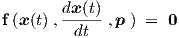
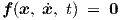
In general, an electronic circuit consisting of arbitrarily controlled elements can be mathematically described by a system of nonlinear first order differential equations1
|
| (2.1) |
with f a vector function. The real-valued2 vector x can represent any mixture of electrical input variables, internal variables and output variables at times t. An electrical variable can be a voltage, a current, a charge or a flux. The real-valued vector p contains all the circuit and device parameters. Parameters may represent component values for resistors, inductors and capacitors, or the width and length of MOSFETs, or any other quantities that are fixed by the particular choice of circuit design and manufacturing process, but that may, at least in principle, be adapted to optimize circuit or device performance. Constants of nature, such as the speed of light or the Boltzmann constant, are therefore not considered as parameters. It should perhaps be explicitly stated, that in this thesis a parameter is always considered to be constant, except for a possible regular updating as part of an optimization procedure that attempts to obtain a desired behaviour for the variables of a system by searching for a suitable set of parameter values.
For practical reasons, such as the crucial model simplicity (to keep the model evaluation times within practical bounds), and to be able to give under certain conditions guarantees on some desirable properties (uniqueness of solution, monotonicity, stability, etc.), we will move away from the general form of Eq. (2.1), and restrict the dependencies to those of layered feedforward neural networks, excluding interactions among different neurons within the same layer. Two subsequent layers are fully interconnected. The feedforward approach allows the definition of nonlinear networks that do not require an iterative method for solving state variables from sets of nonlinear equations (contrary to the situation with most nonlinear electronic circuits), and the existence of a unique solution of network state variables for a given set of network inputs can be guaranteed. As is conventional for feedforward networks, neurons receive their input only from outputs in the layer immediately preceding the layer in which they reside. A net input to a neuron is constructed as a weighted sum, including an offset, of values obtained from the preceding layer, and a nonlinear function is applied to this net input.
However, instead of using only a nonlinear function of a net input, each neuron will now also involve a linear differential equation with two internal state variables, driven by a nonlinear function of the net input, while the net input itself will include time derivatives of outputs from the preceding layer. This enables each single neuron, in concert with its input connections, to represent a second order band-pass type filter, which makes even individual neurons very powerful building blocks for modelling. Together these neurons constitute a dynamic feedforward neural network, in which each neuron still receives input only from the preceding layer. In our new neural network modelling approach, dynamic semiconductor device and subcircuit behaviour is to be modelled by this kind of neural network.
The design of neurons as powerful building blocks for modelling implies that we deliberately support the grandmother-cell concept3 in these networks, rather than strive for a distributed knowledge representation for (hardware) fault-tolerance. Since fault-tolerance is not (yet) an issue in software-implemented neural networks, this is not considered a disadvantage for our envisioned software applications.
The most common modelling situation is that the terminal currents of an electrical device or subcircuit are represented by the outcomes of a model that receives a set of independent voltages as its inputs. This also forms the basis for one of the most prevalent approaches to circuit simulation: Modified Nodal Analysis (MNA) [10]. Less common situations, such as current-controlled models, can still be dealt with, but they are usually treated as exceptions. Although our neural networks do not pertain to any particular choice of physical quantities, we will generally assume that a voltage-controlled model for the terminal currents is required when trying to represent an electronic device or subcircuit by a neural model.
A notable exception is the representation of combinatorial logic, where the relevant inputs and outputs are often chosen to be voltages on the subcircuit terminals in two disjoint sets: one set of terminals for the inputs, and another one for the outputs. This choice is in fact less general, because it neglects loading effects like those related to fan-in and fan-out. However, the representation of combinatorial logic is not further pursued in this thesis, because our main focus is on learning truly analogue behaviour rather than on constructing analogue representations of essentially digital behaviour4.
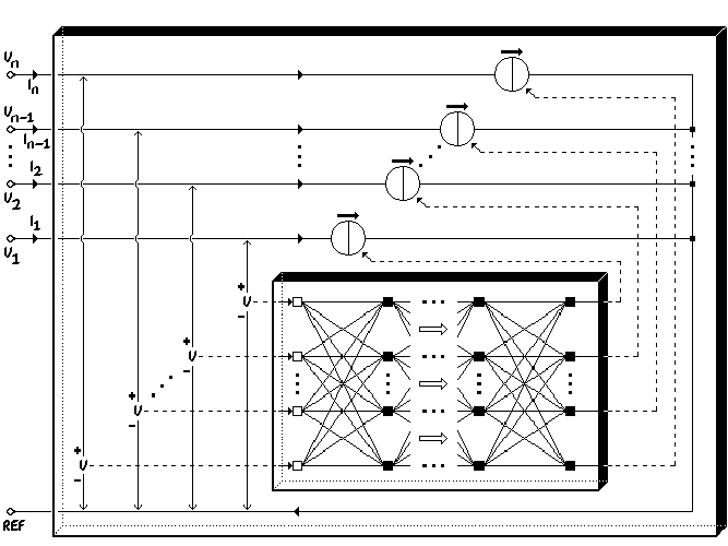
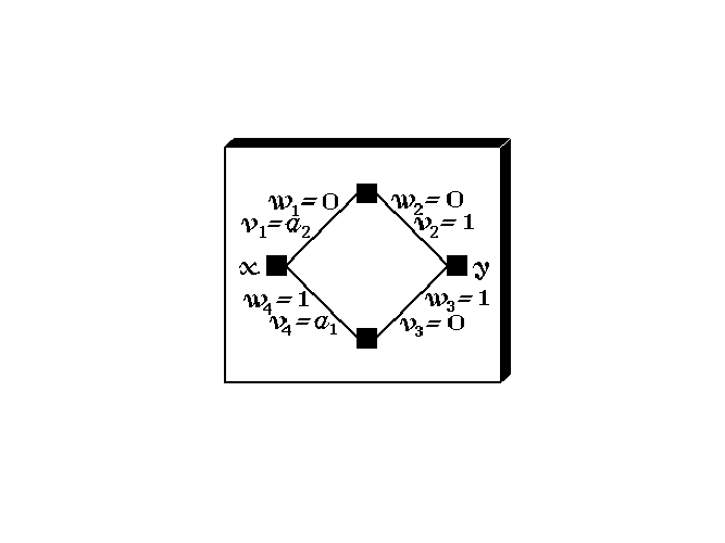
The independent voltages of a voltage-controlled model for terminal currents may be defined w.r.t. some reference terminal. This is illustrated in Fig. 2.1, where n voltages w.r.t. a reference terminal REF form the inputs for an embedded dynamic feedforward neural network. The outputs of the neural network are interpreted as terminal currents, and the neural network outputs are therefore assigned to corresponding controlled current sources of the model for the electrical behaviour of an (n + 1)-terminal device or subcircuit. Only n currents need to be explicitly modelled, because the current through the single remaining (reference) terminal follows from the Kirchhoff current law as the negative sum of the n explicitly modelled currents.
At first glance, Fig. 2.1 may seem to represent a system with feedback. However, this is not really the case, since the information returned to the terminals concerns a physical quantity (current) that is entirely distinct from the physical quantity used as input (voltage). The input-output relation of different physical quantities may be associated with the same set of physical device or subcircuit terminals, but this should not be confused with feedback situations where outputs affect the inputs because they refer to, or are converted into, the same physical quantities. In the case of Fig. 2.1, the external voltages may be set irrespective of the terminal currents that result from them.
In spite of the reduced model (evaluation) complexity, the mathematical notations in the following sections can sometimes become slightly more complicated than needed for a general network description, due to the incorporation of the topological restrictions of feedforward networks in the various derivations.
Before one can write down the equations for dynamic feedforward neural networks, one has to choose a set of labels or symbols with which to denote the various components, parameters and variables of such networks. The notations in this thesis closely follow and extend the notations conventionally used in the literature on static feedforward neural networks. This will facilitate reading and make the dynamic extensions more apparent for those who are already familiar with the latter kind of networks. The illustration of Fig. 2.2 can be helpful in keeping track of the relation between the notations and the neural network components. The precise purpose of some of the notations will only become clear in subsequent sections.
A feedforward neural network will be characterized by the number of layers and the number of
neurons per layer. Layers are counted starting with the input layer as layer 0, such that a
network with output layer K involves a total of K + 1 layers (which would have been K layers in
case one prefers not to count the input layer). Layer k by definition contains Nk neurons, where
k = 0, ,K. The number Nk may also be referred to as the width of layer k. Neurons
that are not directly connected to the inputs or outputs of the network belong to a
so-called hidden layer, of which there are K - 1 in a
,K. The number Nk may also be referred to as the width of layer k. Neurons
that are not directly connected to the inputs or outputs of the network belong to a
so-called hidden layer, of which there are K - 1 in a  -layer network. Network
inputs are labeled as x(0) ≡ (x1(0) ,
-layer network. Network
inputs are labeled as x(0) ≡ (x1(0) , ,xN0(0) )T , and network outputs as x(K) ≡
(x1(K) ,
,xN0(0) )T , and network outputs as x(K) ≡
(x1(K) , ,xNK(K) )T .
The neuron output vector yk ≡ (y1,k , ,yNk,k )T represents the vector of neuron outputs
for layer k, containing as its elements the output variable yi,k for each individual
neuron i in layer k. The network inputs will be treated by a dummy neuron layer
k = 0, with enforced neuron j outputs yj,0 ≡ xj(0), j = 0,
,yNk,k )T represents the vector of neuron outputs
for layer k, containing as its elements the output variable yi,k for each individual
neuron i in layer k. The network inputs will be treated by a dummy neuron layer
k = 0, with enforced neuron j outputs yj,0 ≡ xj(0), j = 0, ,N0. This sometimes
helps to simplify the notations used in the formalism. However, when counting the
number of neurons in a network, we will not take the dummy input neurons into
account.
,N0. This sometimes
helps to simplify the notations used in the formalism. However, when counting the
number of neurons in a network, we will not take the dummy input neurons into
account.
We will apply the convention that separating commas in subscripts are usually left out if this does not cause confusion. For example, a weight parameter wi,j,k may be written as wijk, which represents a weighting factor for the connection from5 neuron j in layer k - 1 to neuron i in layer k. Separating commas are normally required with numerical values for subscripts, in order to distinguish, for example, w12,1,3 from w1,21,3 and w1,2,13 —unless, of course, one has advance knowledge about topological restrictions that exclude the alternative interpretations.
A weight parameter wijk sets the static connection strength for connecting neuron j in layer k - 1 with neuron i in layer k, by multiplying the output yj,k-1 by the value of wijk. An additional weight parameter vijk will play the same role for the frequency dependent part of the connection strength, which is an extension w.r.t. static neural networks. It is a weighting factor for the rate of change in the output of neuron j in layer k - 1, multiplying the time derivative dyj,k-1∕dt by the value of vijk.
In view of the direct association of the extra weight parameter vijk with dynamic behaviour, it is also considered to be a timing parameter. Depending on the context of the discussion, it will therefore be referred to as either a weight(ing) parameter or a timing parameter. As the notation already suggests, the parameters wijk and vijk are considered to belong to neuron i in layer k, which is analogous to the fact that much of the weighted input processing of a biological neuron is performed through its own branched dendrites.
The vector of weight parameters wik ≡ (wi,1,k , ,wi,Nk-1,k )T is conventionally used to
determine the orientation of a static hyperplane, by setting the latter orthogonal to wik. A
threshold parameter θik of neuron i in layer k is then used to determine the position, or offset, of
this hyperplane w.r.t. the origin. Separating hyperplanes as given by wik ⋅yk-1 - θik = 0 are
known to form the backbone for the ability to represent arbitrary static classifications in discrete
problems [36], for example occurring with combinatorial logic, and they can play a similar role
in making smooth transitions among (qualitatively) different operating regions in analogue
applications.
,wi,Nk-1,k )T is conventionally used to
determine the orientation of a static hyperplane, by setting the latter orthogonal to wik. A
threshold parameter θik of neuron i in layer k is then used to determine the position, or offset, of
this hyperplane w.r.t. the origin. Separating hyperplanes as given by wik ⋅yk-1 - θik = 0 are
known to form the backbone for the ability to represent arbitrary static classifications in discrete
problems [36], for example occurring with combinatorial logic, and they can play a similar role
in making smooth transitions among (qualitatively) different operating regions in analogue
applications.
The (generally) nonlinear nature of a neuron will be represented by means of a (generally)
nonlinear function  , which will normally be assumed to be the same function for all neurons
within the network. However, when needed, this is most easily generalized to different
functions for different neurons and different layers, by replacing any occurrence of by
(ik) in every formula in the remainder of this thesis, because in the mathematical
derivations the always concerns the nonlinearity of one particular neuron i in layer
k: it always appears in conjunction with an argument sik that is unique to neuron
i in layer k. For these reasons, it seemed inappropriate to further complicate,
or even clutter, the already rather complicated expressions by using neuron-specific
superscripts for . However, it is useful to know that a purely linear output layer can be
created6,
since that is the assumption underlying a number of theorems on the representational
capabilities of feedforward neural networks having a single hidden layer [19, 23, 34].
, which will normally be assumed to be the same function for all neurons
within the network. However, when needed, this is most easily generalized to different
functions for different neurons and different layers, by replacing any occurrence of by
(ik) in every formula in the remainder of this thesis, because in the mathematical
derivations the always concerns the nonlinearity of one particular neuron i in layer
k: it always appears in conjunction with an argument sik that is unique to neuron
i in layer k. For these reasons, it seemed inappropriate to further complicate,
or even clutter, the already rather complicated expressions by using neuron-specific
superscripts for . However, it is useful to know that a purely linear output layer can be
created6,
since that is the assumption underlying a number of theorems on the representational
capabilities of feedforward neural networks having a single hidden layer [19, 23, 34].
The function is for neuron i in layer k applied to a weighted sum sik of neuron
outputs yj,k-1 in the preceding layer k - 1. The weighting parameters wijk, vijk
and threshold parameter θik take part in the calculation of this weighted sum.
Within a nonlinear function for neuron i in layer k, there may be an additional
(transition) parameter δik , which may be used to set an appropriate scale of change in
qualitative transitions in function behaviour, as is common to semiconductor device
modelling7.
Thus the application of for neuron i in layer k takes the form (sik,δik), which reduces to
(sik) for functions that do not depend on δik.
The dynamic response of neuron i in layer k is determined not only by the timing parameters vijk, but also by additional timing parameters τ1,ik and τ2,ik. Whereas the contributions from vijk amplify rapid changes in neural signals, the τ1,ik and τ2,ik will have the opposite effect of making the neural response more gradual, or time-averaged. In order to guarantee that the values of τ1,ik and τ2,ik will always lie within a certain desired range, they may themselves be determined from associated parameter functions8 τ1,ik = τ1(σ1,ik , σ2,ik) and τ2,ik = τ2(σ1,ik , σ2,ik). These functions will be constructed in such a way that no constraints on the (real) values of the underlying timing parameters σ1,ik and σ2,ik are needed to obtain appropriate values for τ1,ik and τ2,ik.
The differential equation for the output, or excitation, yik of one particular neuron i in layer k > 0 is given by
with the weighted sum s of outputs from the preceding layer
for k > 1, and similarly for the neuron layer k = 1 connected to the network input
which, as stated before, is entirely analogous to having a dummy neuron layer k = 0 with enforced neuron j outputs yj,0 ≡ xj(0). In the following, we will occasionally make use of this in order to avoid each time having to make notational exceptions for the neuron layer k = 1, and we will at times refer to Eq. (2.3) even for k = 1.
The net input sik is analogous to the weighted input signal arriving at the cell body, or soma, of a biological neuron via its branched dendrites, where its value determines whether or not the neuron will fire a signal through its output, the axon, and at what spike rate. Eq. (2.2) can therefore be viewed as the mathematical description of the neuron cell body. In our formalism, we have no analogue of a branched axon, because the branching of the inputs is sufficiently general for the feedforward network topology that we use9.
Finally, to allow for arbitrary network output ranges—because, normally, nonlinear
functions are used that squash the steady state neuron inputs into a finite output
range, such as [0,1] or [-1,1]—the time-dependent outputs yiK of neurons i in the
output layer K yield the network output excitations xi(K) through a linear scaling
transformation
yielding a network output vector x(K).
There is no fundamental reason why a learning scheme would not yield inappropriate values for
the coefficients of the differential terms in a differential equation, which could lead to unstable or
resonant behaviour, or give rise to still other undesirable kinds of behaviour. Even if this occurs
only during the learning procedure, it may at least slow down the convergence towards a
“reasonable” behaviour, whatever we may mean by that, but it may also enhance the probability
of finding an inappropriate local minimum. To decrease the probability of such problems, a
robust software implementation may actually employ functions like τ1,ik  τ1(σ1,ik , σ2,ik) and
τ2,ik
τ1(σ1,ik , σ2,ik) and
τ2,ik  τ2(σ1,ik , σ2,ik) that have any of the relevant—generally nonlinear—constraints built into
the expressions. As a simple example, if τ1,ik = σ1,ik2 and τ2,ik = σ2,ik2, and the
neural network tries to learn the underlying parameters σ1,ik and σ2,ik, then it is
automatically guaranteed that τ1,ik and τ2,ik are not negative. More sophisticated schemes
are required in practice, as will be discussed in section 4.1.2. In the following, the
parameter functions τ1(σ1,ik , σ2,ik) and τ2(σ1,ik , σ2,ik) are often simply denoted by
(timing) “parameters” τ1,ik and τ2,ik, but it must be kept in mind that these are only
indirectly, namely via the σ’s, determined in a learning scheme. Finally, it should be noted
that the τ1,ik have the dimension of time, but the τ2,ik have the dimension of time
squared.
τ2(σ1,ik , σ2,ik) that have any of the relevant—generally nonlinear—constraints built into
the expressions. As a simple example, if τ1,ik = σ1,ik2 and τ2,ik = σ2,ik2, and the
neural network tries to learn the underlying parameters σ1,ik and σ2,ik, then it is
automatically guaranteed that τ1,ik and τ2,ik are not negative. More sophisticated schemes
are required in practice, as will be discussed in section 4.1.2. In the following, the
parameter functions τ1(σ1,ik , σ2,ik) and τ2(σ1,ik , σ2,ik) are often simply denoted by
(timing) “parameters” τ1,ik and τ2,ik, but it must be kept in mind that these are only
indirectly, namely via the σ’s, determined in a learning scheme. Finally, it should be noted
that the τ1,ik have the dimension of time, but the τ2,ik have the dimension of time
squared.
The selection of a proper set of equations for dynamic neural networks cannot be performed through a rigid procedure. Several good choices may exist. The final selection made for this thesis reflects a mixture of—partly heuristic—considerations on desirable properties and “circumstantial evidence” (more or less in hindsight) for having made a good choice. Therefore, we will in the following elaborate on some of the additional reasons that led to the choice of Eqs. (2.2) and (2.3):
with at least two identifiable operating regions provides a general capability
for representing or approximating arbitrary discrete (static) classifications—even for
disjoint sets—using a static (dc) feedforward network and requiring not more than
two hidden layers [36].
also
provides a general capability for representing any continuous multidimensional
(multivariate) static behaviour up to any desired accuracy, using a static feedforward
network and requiring not more than one hidden layer [19, 23]. Recently, it has
even been shown that need only be nonpolynomial in order to prove these
representational capabilities [34]. More literature on the capabilities of neural
networks and fuzzy systems as universal static approximators can be found in
[4, 7, 24, 26, 27, 33].
makes the whole neural
network infinitely differentiable. This is relevant to the accuracy of neural network
models in distortion analyses, but it is also important for the efficiency of the higher
order time integration schemes of an analogue circuit simulator in which the neural
network models will be incorporated.
The complete neuron description from Eqs. (2.2) and (2.3) can act as a (nonlinear) band-pass filter for appropriate parameter settings: the amplitude of the vijk-terms will grow with frequency and dominate the wijk- and θik-terms for sufficiently high frequencies. However, the τ1,ik-term also grows with frequency, leading to a transfer function amplitude on the order of vijk∕τ1,ik, until τ2,ik comes into play and gradually reduces the neuron high-frequency transfer to zero. A band-pass filter approximates the typical behaviour of many physical systems, and is therefore an important building block in system modelling. The non-instantaneous response of a neuron is a consequence of the terms with τ1,ik and τ2,ik.
If all timing parameters in Eqs. (2.2) and (2.3) are zero, i.e., vijk = τ1,ik = τ2,ik = 0, and if one
applies the familiar logistic function  (sik)
(sik)
then one obtains the standard static (not even quasi-static) networks often used with the
popular error backpropagation method, also known as the generalized delta rule, for feedforward
neural networks. Such networks are therefore special cases of our dynamic feedforward
neural networks. The logistic function (sik), as illustrated in Fig. 2.3, is strictly
monotonically increasing in sik. However, we will generally use nonzero v’s and τ’s, and will
instead of the logistic function apply other infinitely smooth (C∞) nonlinear modelling
functions . The standard logistic function lacks the common transition between highly
nonlinear and weakly nonlinear behaviour that is typical for semiconductor devices and
circuits12.
One of the alternative functions for semiconductor device modelling is
with δik≠0. This sigmoid function is strictly monotonically increasing in the variable sik, and
even antisymmetric in sik: 1(sik,δik) = -1(-sik,δik), as illustrated in Fig. 2.4.
Note, however, that the function is
symmetric13
in δik: 1(sik,δik) = 1(sik,-δik). For |δik|≫ 0, Eq. (2.7) behaves asymptotically as
1(sik,δik) ≈-1 + exp(sik + δik)∕|δik| for sik < -|δik|, 1(sik,δik) ≈ sik∕|δik| for
-|δik| < sik < |δik|, and 1(sik,δik) ≈ 1 - exp(δik - sik)∕|δik| for sik > |δik|. The function
defined in Eq. (2.7) needs to be rewritten into several numerically very different but
mathematically equivalent forms for improved numerical robustness, to avoid loss of digits, and
for computational efficiency in the actual implementation. The function is related to the logistic
function in the sense that it is, apart from a linear scaling, the integral over sik of the difference
of two transformed logistic functions, obtained by shifting one logistic function by -δik along
the sik-axis, and another logistic function by +δik. This construction effectively provides us with
a polynomial (linear) region and two exponential saturation regions. Thereby we have the
practical equivalent of two typically dominant basis functions for semiconductor device
modelling, the motivation for which runs along similar lines of thought as in highly
nonlinear multidimensional table modelling [39]. To show the integral relation between
and 1, we first note that the logistic function is related to the tanh function by
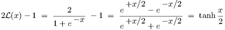
| (2.8) |
The indefinite integral of the tanh(x) function is ln(cosh(x)) (neglecting the integration constant), as is readily verified by differentiating the latter, and we easily obtain
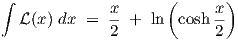
| (2.9) |
such that we find, using the symmetry of the cosh function,
![∫ s
1-- ik(L(x + δ ) - L(x - δ )) dx =
δik 0 ik ik
[ ( ) ( ( ))]sik
1-- x+2-δik-+ ln cosh x+2δik- - x--2δik-+ ln cosh x-2δik- =
δik ⌊ ⌋ 0
cosh x+--δik- sik cosh sik-+-δik-
1--⌈ln-------2---⌉ = -1- ln--------2----
δik cosh x-2-δik- 0 δik cosh sik--2-δik-](thesis19x.png)
|
which is the 1(sik,δik) defined in Eq. (2.7). Another interesting property is that the
1(sik,δik) reduces again to a linearly scaled logistic function for δik approaching zero, i.e.,
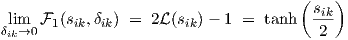
|
The limit is easily obtained by linearizing the integrand in the first line of Eq. (2.10) at x as a function of δik, or alternatively by applying l’Hôpital’s rule.
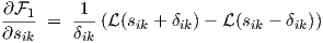
Derivatives of 1(sik,δik) in Eq. (2.7) are needed for transient sensitivity (first partial
derivatives only) and for ac sensitivity (second partial derivatives for dc shift), and are given by
|
![∂2F 1
--21- = ---(L (sik + δik)[1- L (sik + δik)]- L(sik - δik)[1 - L(sik - δik)])
∂sik δik](thesis22x.png)
|

|
![-∂2F1---≡ --∂2F1-- =
∂δik∂(sik ∂sik∂δik )
1-- L(s + δ )[1- L(s + δ )]+ L (s - δ )[1 - L(s - δ )]- ∂F1-
δik ik ik ik ik ik ik ik ik ∂sik](thesis24x.png)
|
The strict monotonicity of 1 is obvious from the expression for the first partial derivative
in Eq. (2.12), since, for positive δik, the first term between the outer parentheses is
always larger than the second term, in view of the fact that is strictly monotonically
increasing. For negative δik, the second term is the largest, but the sign change of
the factor 1∕δik compensates the sign change in the subtraction of terms between
parentheses, such that the first partial derivative of 1 w.r.t. sik is always positive for
δik≠0.
Yet another choice for uses the argument δik only to control the sharpness of the transition
between linear and exponential behaviour, without simultaneously varying the size of the
near-linear interval. Preliminary experience with modelling MOSFET dc characteristics
indicates that this helps to avoid unacceptable local minima in the error function
(cost function) for optimization—unacceptable in the sense that the results show too
gradual near-subthreshold transitions. Another choice for (sik,δik) is therefore defined
as
where the square of δik≠0 avoids the need for absolute signs, while it also keeps practical values
of δik for MOSFET subthreshold and bipolar modelling closer to 1, i.e., nearer to typical values
for most other parameters in a suitably scaled neural network (see also section 4.1.1). For
instance, δik2 ≈ 40 would be typical for Boltzmann factors. The properties of 2
are very similar to those of 1, since it is actually a differently scaled version of 1:

| (2.17) |
So the antisymmetry (in s) and symmetry (in δ) properties still hold for 2. For |δik|≫ 0,
Eq. (2.16) behaves asymptotically as 2(sik,δik) ≈-1 + exp(δik2(sik + 1))∕δik2 for sik < -1,
2(sik,δik) ≈ sik for -1 < sik < 1, and 2(sik,δik) ≈ 1 - exp(-δik2(sik - 1))∕δik2 for sik > 1.
The transitions to and from linear behaviour now apparently lie around sik = -1 and sik = +1,
respectively. The calculation of derivative expressions for sensitivity is omitted here. These
expressions are easily obtained from Eq. (2.17) together with Eqs. (2.12), (2.13), (2.14) and
(2.15). 2(sik,δik) is illustrated in Fig. 2.5.
The functions 0, 1 and 2 are all nonlinear, (strictly) monotonically increasing
and bounded continuous functions, thereby providing the general capability
for representing any continuous multidimensional static behaviour up to any
desired accuracy, using a static feedforward network and requiring not more than
one14
hidden layer [19, 23]. The weaker condition from [34] of having nonpolynomial functions is
then also fulfilled.
Different kinds of dynamic behaviour may arise even from an individual neuron, depending on the values of its parameters. In the following, analytical solutions are derived for the homogeneous part of the neuron differential equation (2.2), as well as for some special cases of the non-homogeneous differential equation. These analytical results lead to conditions that guarantee the stability of dynamic feedforward neural networks. Finally, a few concrete examples of neuron response curves are given.
If the time-dependent behaviour of sik is known exactly (at all time points), the right-hand side of Eq. (2.2) is the source term of a second order ordinary (linear) differential equation in yik. Because sik will be specified at the network input only via values at discrete time points, intermediate values are not really known. However, one could assume and make use of a particular input interpolation, e.g., linear, during each time step. If, for instance, linear interpolation is used, the differential equations of the first hidden layer k = 1 of the neural networks can be solved exactly (analytically) for each time interval spanned by subsequent discrete time points of the network input. If one uses a piecewise linear interpolation of the net input to the next layer, for instance sampled at the same set of time points as given in the network input specification, one can repeat the procedure for the next stages, and analytically solve the differential equations of subsequent layers. This gives a semi-analytic solution of the whole network, where the “semi” refers to the forced piecewise linear shape of the time dependence of the net inputs to neurons.
For each neuron, and for each time interval, we would obtain a differential equation of the form
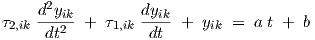
| (2.18) |
with constants a and b for a single segment of the piecewise linear description of the right-hand side of Eq. (2.2). It is assumed here that τ1,ik ≥ 0 and τ2,ik > 0 (the special case τ2,ik = 0 is treated further on).
The homogeneous part (with a = b = 0) can then be written as
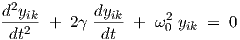
| (2.19) |
for which we have γ ≥ 0 and ω0 > 0, using

| (2.20) |
and

| (2.21) |
The quality factor, or Q-factor, of the differential equation is defined by
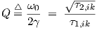
| (2.22) |
Equation (2.19) is solved by substituting yik = exp(λt), giving the characteristic equation
| (2.23) |
with solution(s)
using The “natural frequencies” λ may also be interpreted as eigenvalues, because Eq. (2.19) can be rewritten in the form = Ax with the elements aij of the 2 × 2 matrix A related to γ and ω0
through 2γ = -(a11 + a22) and ω02 = a11a22 - a12a21. Solving the eigenvalue problem
Ax = λIx yields the same solutions for λ as in Eq. (2.24).
= Ax with the elements aij of the 2 × 2 matrix A related to γ and ω0
through 2γ = -(a11 + a22) and ω02 = a11a22 - a12a21. Solving the eigenvalue problem
Ax = λIx yields the same solutions for λ as in Eq. (2.24).
The homogeneous solutions corresponding to Eq. (2.19) fall into several categories [10]:
 )
)
| (2.26) |
with constants C1 and C2, while λ1 = -γ + γd and λ2 = -γ - γd are negative real numbers.
 )
)
| (2.27) |
with constants C1 and C2, while λ1 = λ2 = -γ = -ω0 is real and negative.
 < Q < ∞)
| (2.28) |
with constants C1 and C2, while λ1 = -γ + ȷωd and λ2 = -γ -ȷωd are complex conjugate numbers with a negative real part -γ.
| (2.29) |
with constants C1 and C2, while λ1 = ȷω0 and λ2 = -ȷω0 are complex conjugate imaginary numbers.
A particular solution yik(p)(t) of Eq. (2.18) is given by
| (2.30) |
which is easily verified by substitution in Eq. (2.18).
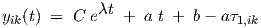
The complete solution of Eq. (2.18) is therefore given by
| (2.31) |
with the homogeneous solution selected from the above-mentioned cases.
In the special case where τ1,ik > 0 and τ2,ik = 0 in (2.18), we have a first order differential equation, leading to
| (2.32) |
with constant C, while λ = -1∕τ1,ik is a negative real number.
From the above derivation it is clear that calculation of the semi-analytical solution, containing exponential, goniometrical and/or square root functions, is rather expensive. For this reason, and because a numerical approach is also easily applied to any alternative differential equation, it is probably better to perform the integration of the second order ordinary (linear) differential equation numerically via discretization with finite differences. The use of the above analytical derivation lies more in providing qualitative insight in the different kinds of behaviour that may occur for different parameter settings. This is particularly useful in designing suitable nonlinear parameter constraint functions τ1,ik = τ1(σ1,ik , σ2,ik) and τ2,ik = τ2(σ1,ik , σ2,ik). The issue will be considered in more detail in section 4.1.2.
The homogeneous differential equation (2.19) is also the homogeneous part of Eq. (2.2).
Moreover, the corresponding analysis of the previous section fully covers the situation where the
neuron inputs yj,k-1 from the preceding layer are constant, such that sik is constant according
to Eq. (2.3). The source term (sik,δik) of Eq. (2.2) is then also constant. In terms of
Eq. (2.18) this gives the constants a = 0 and b = (sik,δik).
If the lossless response of Eq. (2.29) is suppressed by always having τ1,ik > 0 instead of the earlier condition τ1,ik ≥ 0, then the real part of the natural frequencies λ in Eq. (2.24) is always negative. In that case, the behaviour is exponentially stable [10], which here implies that for constant neuron inputs the time-varying part of the neuron output yik(t) will decay to zero as t →∞. The parameter function τ1(σ1,ik , σ2,ik) that will be defined in section 4.1.2.1 indeed ensures that τ1,ik > 0. Due to the feedforward structure of our neural networks, this also means that, for constant network inputs, the time-varying part of the neural network outputs x(K)(t) will decay to zero as t →∞, thus ensuring stability of the whole neural network. This is obvious from the fact that, for constant neural network inputs, the time-varying part of the outputs of neurons in layer k = 1 decays to zero as t →∞, thereby making the inputs to a next layer k = 2 constant. This in turn implies that the time-varying part of the outputs of neurons in layer k = 2 decays to zero as t →∞. This argument is then repeated up to and including the output layer k = K.
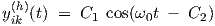
Although the above-derived solutions of section 2.3.1 are well-known classic results, a few illustrations may help to obtain a qualitative overview of various kinds of behaviour for yik(t) that result from particular choices of the net input sik(t). By using a = 0, b = 1, and starting with initial conditions yik = 0 and dyik∕dt = 0 at t = 0, we find from Eq. (2.18) the response to the Heaviside unit step function us(t) given by
Fig. 2.6 illustrates the resulting yik(t) for τ2,ik = 1 and Q ∈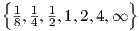 .
.
 .
.
 .
.
One can notice the ringing effects for Q >  , as well as the constant oscillation amplitude for the
lossless case with Q = ∞.
, as well as the constant oscillation amplitude for the
lossless case with Q = ∞.
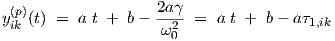
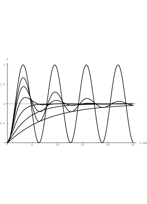
For a = 1, b = 0, and again starting with initial conditions yik = 0 and dyik∕dt = 0 at t = 0, we find from Eq. (2.18) the response to a linear ramp function ur(t) given by
Fig. 2.7 illustrates the resulting yik(t) for τ2,ik = 1 and Q ∈ .
.
From Eqs. (2.30) and (2.31) it is clear that, for finite Q, the behaviour of yik(t) will approach
the delayed (time-shifted) linear behaviour a (t - τ1,ik) + b for t →∞. With the above
parameter choices for τ2,ik and Q, and omitting the case Q = ∞, we obtain the corresponding
delays τ1,ik ∈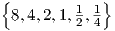 .
.
When the left-hand side of Eq. (2.18) is driven by a sinusoidal source term (instead of the present source term a t + b), we may also represent the steady state behaviour by a frequency domain transfer function H(ω) as given by
| (2.35) |
which for τ2,ik = 1 and Q ∈ results in the plots for
  and
and  H as shown in
Fig. 2.8 and Fig. 2.9, respectively. Large peaks in
H as shown in
Fig. 2.8 and Fig. 2.9, respectively. Large peaks in  arise for large values of Q. These peaks
are positioned near angular frequencies ω = ω0, and their height approximates the
corresponding value of Q. The curve in Fig. 2.9 that gets closest to a 180 degree phase
shift is the one corresponding to Q = 4. At the other extreme, the curve that hardly
gets beyond a 90 degree phase shift corresponds to Q =
arise for large values of Q. These peaks
are positioned near angular frequencies ω = ω0, and their height approximates the
corresponding value of Q. The curve in Fig. 2.9 that gets closest to a 180 degree phase
shift is the one corresponding to Q = 4. At the other extreme, the curve that hardly
gets beyond a 90 degree phase shift corresponds to Q =  . For Q = 0 (not shown),
the phase shift of the corresponding first order system would never get beyond 90
degrees.
. For Q = 0 (not shown),
the phase shift of the corresponding first order system would never get beyond 90
degrees.
Frequency domain transfer functions of individual neurons and transfer matrices of neural networks will be discussed in more detail in the context of small-signal ac analysis in sections 3.2.1.1 and 3.2.3.
Decisive for a widespread application of dynamic neural networks will be the ability of these networks to represent a number of important general classes of behaviour. This issue is best considered separate from the ability to construct or learn a representation of that behaviour. As in mathematics, a proof of the existence of a solution to a problem does not always provide the capability to find or construct a solution, but it at least indicates that it is worth trying.
In physical modelling for circuit simulation, a device is usually partitioned into submodels or lumps that are described quasistatically, which implies that the electrical state of such a part responds instantaneously to the applied bias. In other words, one considers submodels that themselves have no internal nodes with associated charges.
One of the most common situations for a built-in circuit simulator model is that dc terminal currents I(dc) and so-called equivalent terminal charges Q(eq) of a device are directly and uniquely determined by the externally applied time-dependent voltages V (t). This is also typical for the quasistatic modelling of the intrinsic behaviour of MOSFETs, in order to get rid of the non-quasistatic channel charge distribution [48]. The actual quasistatic terminal currents of a device model with parameters p are then given by
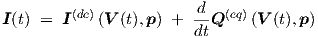
| (2.36) |
In MOSFET modelling, one often uses just one such a quasistatic lump. For example, the Philips’ MOST model 9 belongs to this class of models. The validity of a single-lump quasistatic MOSFET model will generally break down above angular frequencies that are larger than the inverse of the dominant time constants of the channel between drain and source. These time constants strongly depend on the MOSFET bias condition, which makes it difficult to specify one characteristic frequency15. However, because a quasistatic model can correctly represent the (dc+capacitive) terminal currents in the low-frequency limit, it is useful to consider whether the neural networks can represent (the behaviour of) arbitrary quasistatic models as a special case, namely as a special case of the truly dynamic non-quasistatic models. Fortunately, they can.
In the literature it has been shown that continuous multidimensional static behaviour can up to any desired accuracy be represented by a (linearly scaled) static feedforward network, requiring not more than one hidden layer and some nonpolynomial function [19, 23, 34]. So this immediately covers any model function for the dc terminal current I(dc)(V ). Furthermore, simply by adding another network in parallel, one can of course also represent any function Q(eq)(V ) with a neural network containing not more than one hidden layer. However, according to Eq. (2.36), we must add the time-derivative of Q(eq) to the dc current I(dc). This is easily done with an additional network layer k = 3. A number of nonzero wij,3 and zero vij,3 values are used to copy the dc currents into the net input si,3 of output neurons in this extra layer. Zero wij,3 and nonzero vij,3 values are used to add the appropriate time derivatives of the charges, as given by the outputs of other neurons in layer k = 2—those of the previously mentioned parallel network.
An illustration of the procedure is given in Fig. 2.10 for a 3-input 3-output neural network, as
needed to represent a quasistatic model for a 4-terminal device. (We will not try to formalize
and prescribe the rather trivial bookkeeping details of giving concrete values to the wij,3 and
vij,3.) The τ1,ik and τ2,ik parameters are kept at zero in all layers. The net input of output layer
k = 3 is already the desired outcome of Eq. (2.36) and must therefore be transparently passed
on to the network outputs by using linear(ized) behaviour in . The latter is always possible by
making appropriate use of the linear scalings that are part of our neural network
definitions. A (nearly) linear region of need not explicitly be present, as in 2.
Equivalent linear behaviour can be obtained up to any desired accuracy from any
continuous , by scaling the wij,3 and vij,3 values by a sufficiently small factor, and
compensating this scaling at the network output by a corresponding unscaling, by
multiplying the αi values with the inverse of this factor. The θi,3 and βi can all be kept at
zero.
This very simple constructive procedure shows that all quasistatic models are representable up to arbitrary accuracy by our class of dynamic neural networks. It does not exclude the possibility that the same may also be possible with fewer than two hidden layers.
In this section we show that with our dynamic neural network definitions Eqs. (2.2), (2.3) and (2.5), the behaviour of any linear time invariant lumped circuit with frequency transfer matrix H(s) can be represented exactly. Here s is the Laplace variable, also called the complex frequency.
We will first restrict the discussion to the representation of a single but arbitrary element H(s) of the transfer matrix H(s). The H(s) for multi-input, multi-output systems can afterwards be synthesized by properly merging and/or extending the neural networks for individual elements H(s).
It is known that the behaviour of any uniquely solvable linear time-invariant lumped circuit can be characterized by the ratio of two polynomials in s with only real-valued coefficients [10]. Writing the nominator polynomial as n(s) and the denominator polynomial as d(s), we therefore have
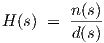
| (2.37) |
The zeros of d(s) are called the poles of H(s), and they are the natural frequencies of the system characterized by H(s). The zeros of n(s) are also the zeros of H(s). Once the poles and zeros of all elements of H(s) are known or approximated, a constructive mapping can be devised which gives an exact mapping of the poles and zeros onto our dynamic feedforward neural networks.
It is also known that all complex-valued zeros of a polynomial with real-valued coefficients occur in complex conjugate pairs. That implies that such a polynomial can always be factored into a product of first or second degree polynomials with real-valued coefficients. Once these individual factors have been mapped onto equivalent dynamic neural subnetworks, the construction of their overall product is merely a matter of putting these subnetworks in series (cascading).
As shown further on, the subnetworks will consist of one or at most three linear dynamic
neurons. W.r.t. a single input j, a linear dynamic neuron—with (sik) = sik —has a transfer
function hijk(s) of the form
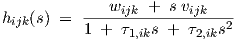
| (2.38) |
as follows from the replacement by the Laplace variable s of the time differentiation operator d∕dt in Eqs. (2.2) and (2.3).
In the following, it is assumed that H(s) is coprime, meaning that any common factors in the nominator and denominator of H(s) have already been cancelled.
In principle, a pole at the origin of the complex plane could exist. However, that would create a factor 1∕s in H(s), which would remain after partial fraction expansion as a term proportional to 1∕s, having a time domain transform corresponding to infinitely slow response. This follows from the inverse Laplace transform of 1∕(s + a): exp(-at), with a positive real, and taking the limit a ↓ 0. See also [10]. That would not be a physically interesting or realistic situation, and we will assume that we do not have any poles located exactly at the origin of the complex plane. Moreover, it means that any constant term in d(s) —because it now will be nonzero—can be divided out, such that H(s) is written in a form having the constant term in d(s) equal to 1, and with the constant term in n(s) equal to the static (dc) transfer of H(s), i.e., H(s = 0).
Apparently we can represent any complex conjugate pair of poles of H(s), using just a single neuron.
To ensure stability, we may again want non-positive real parts in both (real) poles, i.e., a1 ≤ 0, a2 ≤ 0, such that together with the exclusion of the origin (0,0), τ1,ik > 0, and also τ2,ik > 0. For a1 ≡ a2, the same values for τ1,ik and τ2,ik arise as in the case with complex conjugate zeros (a ± ȷb) with b ≡ 0, which is what one would expect.
Apparently we can represent two arbitrary real poles of H(s), using just a single neuron.
For stability, we will want non-positive real parts for the (real) pole (a,0), i.e., a ≤ 0, such that together with the exclusion of the origin (0,0), τ1,ik > 0.
Apparently we can represent a single arbitrary real pole of H(s), using just a single neuron.
This provides us with all the ingredients needed to construct an arbitrary set of poles for the transfer function H(s) of an electrical network. Any set of poles of H(s) can now be represented by cascading a number of neurons.
It should be noted that many pole orderings, e.g., with increasing distance from the origin, may give an arbitrary sequence of real poles and complex conjugate poles. Since a pair of complex conjugate poles must be covered by one and the same neuron, due to its real coefficients, one generally has to do some reordering to avoid having, for instance, one real pole, followed by a pair of complex conjugate poles, followed by a real pole again: the two real poles have to be grouped together to align them with the two neurons needed to represent the two real poles and the pair of complex conjugate poles, respectively.
The individual zeros of the nominator n(s) of H(s) can in general not be covered by associated single neurons of the type defined by Eqs. (2.2) and (2.3). The reason is that the zero of a single-input neuron is found from wijk + svijk = 0, i.e, s = -wijk∕vijk, while wijk and vijk are both real. Consequently, a single single-input neuron can only represent an arbitrary real-valued zero a of n(s), i.e., a factor (s - a), by taking vijk≠0 and wijk = -avijk. The real-valued wijk and vijk of a single neuron do not allow for complex-valued zeros of n(s).
However, arbitrary complex-valued zeros can be represented by using a simple combination of three neurons, with two of them in parallel in a single layer, and a third neuron in the next layer receiving its input from the other two neurons. The two parallel neurons share their single input. With this neural subnetwork we shall be able to construct an arbitrary factor 1 + a1s + a2s2 in n(s), with a1, a2 both real-valued. This then covers any possible pair of complex conjugate zeros16. It is worth noting that in the representation of complex-valued zeros, one still ends up with one modelled zero per neural network layer, but now using three neurons for two zeros instead of two neurons for two (real) zeros.
First we relabel, for notational clarity, the wijk and vijk parameters of the single-input (x) single-output (y) neural subnetwork as indicated in Fig. 2.11.
If we neglect, for simplicity of discussion, the poles by temporarily17 setting all the τ1,ik and τ2,ik of the subnetwork equal to zero, then the transfer of the subnetwork is obviously given by (w1 + v1s)(w2 + v2s) + (w3 + v3s)(w4 + v4s). Setting w1 = 0, v1 = a2, w2 = 0 and v2 = 1 yields a term a2s2 in the transfer, and setting w4 = 1, v4 = a1, w3 = 1 and v3 = 0 yields another term 1 + a1s in the transfer. Together this indeed gives the above-mentioned arbitrary factor 1 + a1s + a2s2 with a1, a2 both real-valued. Similar to the earlier treatment of complex conjugate poles (a ± ȷb) with a and b both real, we find that the product of s - (a + ȷb) and s - (a - ȷb) after division by a2 + b2 leads to a factor 1 - [2a∕(a2 + b2)]s + [1∕(a2 + b2)]s2. This exactly matches the form 1 + a1s + a2s2 if we take
Any set of zeros of H(s) can again be represented by cascading a number of neurons—or neural subnetworks for the complex-valued zeros.The constant term in n(s) remains to be represented, since the above assignments only lead to the correct zeros of H(s), but with a constant term still equal to 1, which will normally not match the static transfer of H(s). The constant term in n(s) may be set to its proper value by multiplying the wijk and vijk in one particular layer of the chain of neurons by the required value of the static (real-valued) transfer of H(s).
One can combine the set of poles and zeros of H(s) in a single chain of neurons, using only one neuron per layer except for the complex zeros of H(s), which lead to two neurons in some of the layers. One can make use of neurons with missing poles by setting τ1,ik = τ2,ik = 0, or make use of neurons with zeros by setting vijk = 0, in order to map any given set of poles and zeros of H(s) onto a single chain of neurons.
Multiple H(s)-chains of neurons can be used to represent each of the individual elements of the H(s) matrix of multi-input, multi-output linear systems, while the wijK of an (additional) output layer K, with vijK = 0 and αi = 1, can be used to finally complete the exact mapping of H(s) onto a neural network. A value wijK = 1 is used for a connection from the chain for one H(s)-element to the network output corresponding to the row-index of that particular H(s)-element. For all remaining connections wijK = 0.
It should perhaps be stressed that most of the proposed parameter assignments for poles and zeros are by no means unique, but merely serve to show, by construction, that at least one exact pole-zero mapping onto a dynamic feedforward neural network exists. Any numerical reasons for using a specific ordering of poles or zeros, or for using other alternative combinations of parameter values were also not taken into account. Using partial fraction expansion, it can also be shown that a neural network with just a single hidden layer can up to arbitrary accuracy represent the behaviour of linear time-invariant lumped circuits, assuming that all poles are simple (i.e., non-identical) poles and that there are more poles than zeros. The former requirement is in principle easily fulfilled when allowing for infinitesimal changes in the position of poles, while the latter requirement only means that the magnitude of the transfer should drop to zero for sufficiently high frequencies, which is often the case for the parts of system behaviour that are relevant to be modelled18.
Although learning in neural networks with feedback is not covered in this thesis, it is worthwhile to consider the ability to represent certain kinds of behaviour when feedback is applied externally to our neural networks. As it turns out, the addition of feedback allows for the representation of very general classes of both linear and nonlinear multidimensional dynamic behaviour.
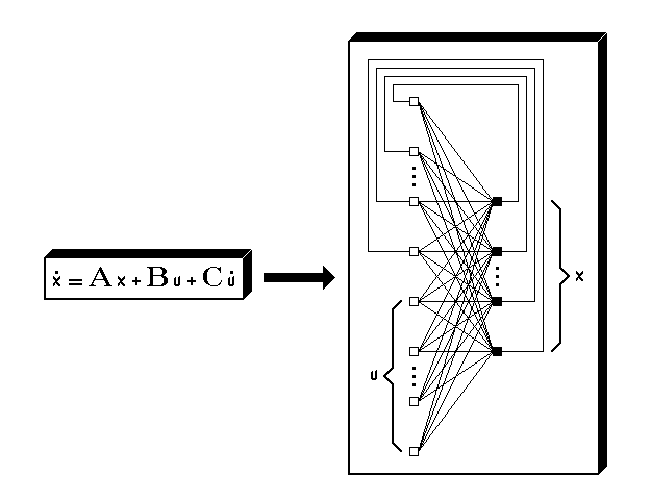
We will show in this section that with definitions in Eqs. (2.2), (2.3) and (2.5), a dynamic feedforward neural network without a hidden layer but with external feedback suffices to represent the time evolution of any linear dynamic system characterized by the state equation

| (2.43) |
where A is an n × n matrix, x is a state vector of length n, B and C are n × m matrices, and
u = u(t) is an explicitly time-dependent input vector of length m. As usual, t represents
the time. First derivatives w.r.t. time are now indicated by a dot, i.e.,  ≡ dx∕dt,
 ≡ du∕dt.
Eq. (2.43) is a special case of the nonlinear state equation

| (2.44) |
with nonlinear vector function f. This form is already sufficiently general for circuit simulation with quasistatically modelled (sub)devices, but sometimes the even more general implicit form
| (2.45) |
is used in formal derivations. The elements of x are in all these cases called state variables.
However, we will at first only further pursue the representation of linear dynamic systems by
means of neural networks. We will forge equation Eq. (2.43) into a form corresponding to a
feedforward network having a  topology, supplemented by direct external
feedback from all n outputs to the first n (of a total of n + m) inputs. The remaining m
network inputs are then used for the input vector u(t). This is illustrated in Fig. 2.12.
topology, supplemented by direct external
feedback from all n outputs to the first n (of a total of n + m) inputs. The remaining m
network inputs are then used for the input vector u(t). This is illustrated in Fig. 2.12.
By defining matrices
| (2.46) |

| (2.47) |

| (2.48) |

| (2.49) |
with I the n × n identity matrix, we can rewrite Eq. (2.43) into a form with nonsquare n × (n + m) matrices as in
|
The elements of the right-hand side x of Eq. (2.50) can be directly associated with the neuron
outputs yi,1 in layer k = 1. We set αi = 1 and βi = 0 in Eq. (2.5), thereby making the network
outputs identical to the neuron outputs. Due to the external feedback, the elements of x in
Eq. (2.50) are now also identical to the network inputs xi(0), i = 0,…,n - 1. To complete the
association of Eq. (2.50) with Eqs. (2.2) and (2.3), we take (sik) ≡ sik. The wij,1 are simply
the elements of the matrix  in the first term in the left-hand side of Eq. (2.50), while
the vij,1 are the elements of the matrix
in the first term in the left-hand side of Eq. (2.50), while
the vij,1 are the elements of the matrix  in the second term in the left-hand side of
Eq. (2.50). Through these choices, we can put the remaining parameters to zero, i.e., τ1,i,1 = 0,
τ2,i,1 = 0 and θi,1 = 0 for i = 0,…,n - 1, because we do not need these parameters
here.
in the second term in the left-hand side of
Eq. (2.50). Through these choices, we can put the remaining parameters to zero, i.e., τ1,i,1 = 0,
τ2,i,1 = 0 and θi,1 = 0 for i = 0,…,n - 1, because we do not need these parameters
here.
This short excursion into feedforward neural networks with external feedback already shows, that our present set of neural network definitions has a great versatility. Very general linear dynamic systems are easily mapped onto neural networks, with only a minimal increase in representational complexity, the only extension being the constraints imposed by the external feedback.
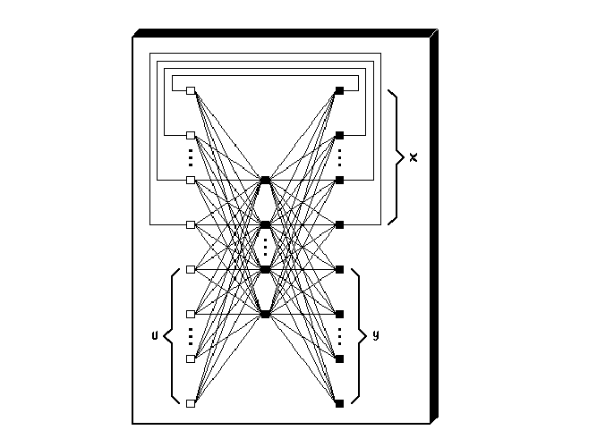
The results of the preceding section give rise to the important question, whether we can also devise a procedure that allows us, at least in principle, to represent arbitrary nonlinear dynamic systems as expressed by Eq. (2.45). That would imply that our feedforward neural networks, when supplemented with feedback connections, can represent the behaviour of any nonlinear dynamic electronic circuit.
We will consider the neural network of Fig. 2.13.
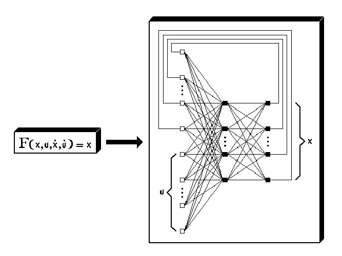
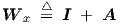
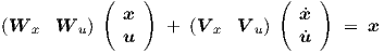
As in the preceding section, we will use a state vector x of length n in a feedback loop, thereby forming part of the network input, while u = u(t) is the explicitly time-dependent input vector of length m. All timing parameters τ1,i,1, τ2,i,1 τ1,i,2, τ2,i,2 and vij,2 are kept at zero, because it turns out that we do not need them to answer the above-mentioned question. Only the timing parameters vij,1 of the hidden layer k = 1 will generally be nonzero. We denote the net input to layer k = 1 by a vector s of length p, with elements si,1. Similarly, the threshold vector θ of length p contains elements θi,1. Then we have
|
or, alternatively,
|
with Wx the n × p matrix of weight parameters wij,1 associated with input vector x, V x the n × p matrix of weight parameters vij,1 associated with input vector x, Wu the m × p matrix of weight parameters wij,1 associated with input vector u, and V u the m × p matrix of weight parameters vij,1 associated with input vector u.
The latter form of Eq. (2.52) is also obtained if one considers a regular static neural network
with input weight matrix W = 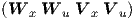 , if the complete vector
  T is
supposed to be available at the network input.
T is
supposed to be available at the network input.
This mathematical equivalence allows us to immediately exploit an important
result from the literature on static feedforward neural networks. From the work of
[19, 23, 34], it is clear that we can represent at the network output any continuous
nonlinear vector function F up to arbitrary accuracy, by requiring just
one hidden layer with nonpolynomial functions —and with linear or effectively
linearized19
functions in the output layer.
up to arbitrary accuracy, by requiring just
one hidden layer with nonpolynomial functions —and with linear or effectively
linearized19
functions in the output layer.
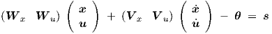
We will assume that F has n elements, such that the feedback yields
|
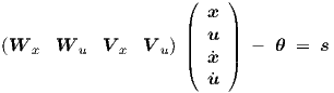
In order to represent Eq. (2.45), we realize that the explicitly time-dependent, but still unspecified, inputs u = u(t) allow us to define a function F as
|
where the arguments x,  and t should now be viewed as independent variables in this
definition, and where appropriate choices for u(t) make it possible to represent any explicitly
time-dependent parts of f.
and t should now be viewed as independent variables in this
definition, and where appropriate choices for u(t) make it possible to represent any explicitly
time-dependent parts of f.
The above approximation can be made arbitrarily close, such that substitution of Eq. (2.54) in Eq. (2.53) indeed yields the general state equation (2.45), i.e.,

|
It should be clear that there is a major semantic distinction between a function definition like (2.54), which should in principle hold for any combination of argument values to have a nontrivial mapping that fully covers the characteristics of the system to be modelled, and relations between functions, such as (2.45) and (2.53), which pose implicit relations among—hence restrictions to—argument values.
Until now, we only considered state equations, while a complete analysis of arbitrary nonlinear
dynamic systems also involves output equations for nonstate variables of the form
y = G , also known as input-state-output equations or read-out map according to [9].
These equations relate the state variables to the observables. However, with electronic
circuits the distinction between the two is often blurred, since output functions, e.g.,
for currents, may already be part of the construction—and solution—of the state
equations, e.g., for voltages. As long as one is only concerned with charges, fluxes,
voltages and currents, the output functions are often components of f
, also known as input-state-output equations or read-out map according to [9].
These equations relate the state variables to the observables. However, with electronic
circuits the distinction between the two is often blurred, since output functions, e.g.,
for currents, may already be part of the construction—and solution—of the state
equations, e.g., for voltages. As long as one is only concerned with charges, fluxes,
voltages and currents, the output functions are often components of f . For
example, it may be impossible to solve the nodal voltages in a circuit without evaluating
the terminal currents of devices, because these take part in the application of the
Kirchhoff current law. Therefore, in electronic circuit analysis, the output equations G are
often not considered as separate equations, and only Eq. (2.45) is considered in the
formalism.
. For
example, it may be impossible to solve the nodal voltages in a circuit without evaluating
the terminal currents of devices, because these take part in the application of the
Kirchhoff current law. Therefore, in electronic circuit analysis, the output equations G are
often not considered as separate equations, and only Eq. (2.45) is considered in the
formalism.
Any left-over output equations could be represented by a companion feedforward neural network
with one hidden layer, but without external feedback. The additional network takes the available
x and u as its inputs, and emulates the behaviour of a static feedforward neural network
with inputs x, u and  through use of the parameters vij,1. The procedure would
be entirely analogous to the mathematical equivalence that we used earlier in this
section.
through use of the parameters vij,1. The procedure would
be entirely analogous to the mathematical equivalence that we used earlier in this
section.
Furthermore, since x is, due to the feedback, also available at the input of the network in
Fig. 2.13, the companion network for G can be placed in parallel with the network
representing F, thereby still having only one hidden layer for the combination of the two
neural networks. This in turn implies that the two neural networks (for  and for
  )
can be merged into one neural network with the same functionality, as is shown in
Fig. 2.14.
)
can be merged into one neural network with the same functionality, as is shown in
Fig. 2.14.
In view of all these very general results, the design of learning procedures for feedforward nonlinear dynamic neural networks with external feedback connections could be an interesting topic for future work on universal approximators for dynamic systems. On the other hand, feedback will definitely reduce the tractability of giving mathematical guarantees on several desirable properties like uniqueness of behaviour (i.e., no multiple solutions to the network equations), stability, and monotonicity. The representational generality of dynamic neural networks with feedback basically implies, that any kind of unwanted behaviour may occur, including, for instance, chaotic behaviour. Furthermore, feedback generally renders it impossible to obtain explicit expressions for nonlinear behaviour, such that nonconvergence may occur during numerical simulation.
For the present, the value of the above considerations lies mainly in establishing links with general circuit and system theory, thus helping us understand how our non-quasistatic feedforward neural networks constitute a special class within a broader, but also less tractable, framework. We have been considering general continuous-time neural systems. Heading in the same general direction is a recent publication on the abilities of continuous-time recurrent neural networks [20]. Somewhat related work on general discrete-time neural systems in the context of adaptive filtering can be found in [41].
Apart from the intrinsic capabilities of neural networks to represent certain classes of behaviour, as discussed before, it is also important to consider the possibilities of mapping these neural networks onto the input languages of existing analogue circuit simulators. If that can be done, one can simulate with neural network models without requiring the implementation of new built-in models in the source code of a particular circuit simulator. The fact that one then does not need access to the source code, or influence the priority settings of the simulator release procedures, is a major advantage. The importance of this simulator independence is the reason to consider this matter before proceeding with the more theoretical development of learning techniques, described in Chapter 3. For brevity, only a few of the more difficult or illustrative parts of the mappings will be explained in detail, although examples of complete mappings are given in Appendix C, sections C.1 and C.2.
In the following, it will be shown how several neuron nonlinearities can be represented by electrical circuits containing basic semiconductor devices and other circuit elements, when using idealized models that are available in almost any circuit simulator, for instance in Berkeley SPICE. This allows the use of neural models in most existing analogue circuit simulators.
2It is worth noting that Eq. (2.16) can be rewritten as a combination of ideal diode functions and their inverses20 through
withIf the junction emission coefficient of an ideal diode is set to one, and if we denote the thermal voltage by V t, the diode expressions become
| (2.58) |
which can then be used to represent Eq. (2.56) for a single
temperature21.
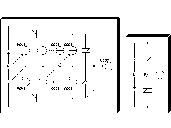
This need for only basic semiconductor device expressions can be seen as another,
though qualitative, argument in favour of the choice of functions like 2 for
semiconductor device modelling purposes. It can also be used to map neural network
descriptions onto primitive (non-behavioural, non-AHDL) simulator languages
like the Berkeley SPICE input language: only independent and linear controlled
sources22,
and ideal diodes, are needed to accomplish that for the nonlinearity 2, as is outlined in the left
part of Fig. 2.15. Cadence Spectre is largely compatible with Berkeley SPICE, and can therefore
be used as a substitute for SPICE.
The logistic function of Eq. (2.6) can also be mapped onto a SPICE representation, for
example via
| (2.59) |
where I is the current through a series connection of two identical ideal diodes, having the cathodes wired together at an internal node with voltage V 0. V is here the voltage across the series connection. When expressed in formulas, this becomes

| (2.60) |
from which V 0 can be analytically solved as
| (2.61) |
which, after substitution in Eq. (2.60), indeed yields a current I that relates to the logistic function of Eq. (2.6) according to Eq. (2.59).
However, in a typical circuit simulator, the voltage solution V 0 is obtained by a numerical
nonlinear solver (if it converges), applied to the nonlinear subcircuit involving the series
connection of two diodes, as is illustrated in the right part of Fig. 2.15. Consequently, even
though a mathematically exact mapping onto a SPICE-level description is possible,
and even though an analytical solution for the voltage V 0 on the internal node is
known (to us), numerical problems in the form of nonconvergence of Berkeley SPICE
and Cadence Spectre could be frequent. This most likely applies to the SPICE input
representations of both 2 and the logistic function . With Pstar, this problem is
avoided, because one can explicitly define the nonlinear expressions for 2 and in
the input language of Pstar. For 2, this will be shown in the next section, together
with the Pstar representation of several other components of the neuron differential
equation.
An example of a complete SPICE neural network description can be found in Appendix C, section C.2. That example includes the representation of the full neuron differential equation (2.2) and the connections among neurons corresponding to Eq. (2.3). The left-hand side of Eq. (2.2) is represented in a way that is very similar to the Pstar representation discussed in the next section. The terms with time derivatives in Eq. (2.3) are obtained from voltages induced by currents that are forced through linear inductors.
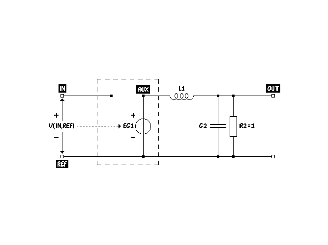
When generating analogue behavioural models for circuit simulators, one normally has to map the neuron cell body, or soma, differential equation (2.2) onto some equivalent electrical circuit. Because the Pstar input language is among the most powerful and readable, we will here consider a Pstar description, a so-called user model, for a single non-quasistatic neuron, according to the circuit schematic as shown in Fig. 2.16.
The neuron model is specified in the following example of a so-called user-defined model, which simply means a model described in the Pstar input language:
A few comments will clarify the syntax for those who are not familiar with the Pstar input
language. Connecting (terminal) nodes are indicated by unique symbolic names between
parentheses, like in (IN,OUT,REF). The neuron description Eq. (2.2) is encapsulated in a user
model definition, which defines the model Neuron, having terminal nodes IN, OUT, and a
reference terminal called REF. The neuron net input sik will be represented by the
voltage across nodes IN and REF, while the neuron output yik will be represented
by the voltage across OUT and REF. The neuron parameters delta= δik, tau1=τ1,ik
and tau2=τ2,ik enter as model arguments as specified in the first line, and are in
this example all supposed to be nonzero. Intermediate parameters can be defined,
as in delta2= δik2. The nonlinearity 2(sik,δik) is represented via a nonlinearly
controlled voltage source EC1, connected between an internal node AUX and the reference
node REF. EC1 is controlled by (a nonlinear function of) the voltage between nodes
IN and REF. 2 was rewritten in terms of exponential functions exp() instead of
hyperbolic cosines, because Pstar does not know the latter. Contrary to SPICE, Pstar
does not require a separate equivalent electrical circuit to construct the nonlinearity
2.
The voltage across EC1 represents the right-hand side of Eq. (2.2). A linear inductor L1 with inductance tau1 connects internal node AUX and output node OUT, while OUT and REF are connected by a second linear capacitor C2 with capacitance tau2/tau1, in parallel with a linear resistor R2 of 1.0 ohm.
It may not immediately be obvious that this additional circuitry does indeed represent the
left-hand side of Eq. (2.2). To see this, one first realizes that the total current flowing through
C2 and R2 is given by yik + tau2/tau1  , because the neuron output yik is the voltage
across OUT and REF. If only a zero load is externally connected to output node OUT
(which can be ensured by properly devising an encapsulating circuit model for the
whole network of neurons), all this current has to be supplied through the inductor
L1. The flux Φ through L1 therefore equals its inductance tau1 multiplied by this
total current, i.e., tau1 yik + tau2
, because the neuron output yik is the voltage
across OUT and REF. If only a zero load is externally connected to output node OUT
(which can be ensured by properly devising an encapsulating circuit model for the
whole network of neurons), all this current has to be supplied through the inductor
L1. The flux Φ through L1 therefore equals its inductance tau1 multiplied by this
total current, i.e., tau1 yik + tau2  . Furthermore, the voltage induced across
this inductor is given by the time derivative of the flux, giving tau1
. Furthermore, the voltage induced across
this inductor is given by the time derivative of the flux, giving tau1  + tau2
 . This voltage between AUX and OUT has to be added to the voltage yik between
OUT and REF to obtain the voltage between AUX and REF. The sum yields the entire
left-hand side of Eq. (2.2). However, the latter voltage must also be equal to the
voltage across the controlled voltage source EC1, because that source is connected
between AUX and REF. Since we have already ensured that the voltage across EC1
represents the right-hand side of Eq. (2.2), we now find that the left-hand side of
Eq. (2.2) has to equal the right-hand side of Eq. (2.2), which implies that the behaviour
of our equivalent circuit is indeed consistent with the neuron differential equation
(2.2).
. This voltage between AUX and OUT has to be added to the voltage yik between
OUT and REF to obtain the voltage between AUX and REF. The sum yields the entire
left-hand side of Eq. (2.2). However, the latter voltage must also be equal to the
voltage across the controlled voltage source EC1, because that source is connected
between AUX and REF. Since we have already ensured that the voltage across EC1
represents the right-hand side of Eq. (2.2), we now find that the left-hand side of
Eq. (2.2) has to equal the right-hand side of Eq. (2.2), which implies that the behaviour
of our equivalent circuit is indeed consistent with the neuron differential equation
(2.2).
The neuron net input sik in Eq. (2.3), represented by the voltage across nodes IN and REF, can be constructed at a higher hierarchical level, the neural network level, of the Pstar description. The details of that rather straightforward construction are omitted here. It only involves linear controlled sources and linear inductors. The latter are used to obtain the time derivatives of currents in the form of induced voltages, thereby incorporating the differential terms of Eq. (2.3). An example of a complete Pstar neural network description can be found in Appendix C, section C.1.
The dynamic feedforward neural networks as specified by Eqs. (2.2), (2.3) and (2.5), were designed to have a number of attractive numerical and mathematical properties. There is a certain price to be paid, however.
The fact that the neural networks are guaranteed to have a unique dc solution immediately implies that the behaviour of a circuit having multiple dc solutions cannot be completely modelled by a single neural network, indiscriminate of our time domain extensions. An example is the nonlinear resistive flip-flop circuit, which has two stable dc solutions—and one metastable dc solution that we usually don’t (want to) see. Circuits like these are called bistable. Because the neural networks can represent any (quasi)static behaviour up to any required accuracy, multiple solutions can be obtained by interconnecting the neural networks, or their corresponding electrical behavioural models, with other circuit components or other neural networks, and by imposing (some equivalent of) the Kirchhoff current law. After all, in regular circuit simulation, including time domain and frequency domain simulation, all electronic circuits are represented by interconnected (sub)models that are themselves purely quasistatic. Nevertheless, this solves the problem only in principle, not in practice, because it assumes that one already knows how to properly decompose a circuit and how to characterize the resulting “hidden” components by training data. In general, one does not have that knowledge, which is why a black-box approach was advocated in the first place.
The multiple dc solutions of the bistable flip-flop arise from feedback connections. Since there are no feedback connections within the neural networks, modelling limitations will turn up in all cases where feedback is essential for a certain dc behaviour. This does definitely not mean that our feedforward neural networks cannot represent devices and subcircuits in which some form of feedback takes place. If the feedback results in unique dc behaviour in all situations, or if we want to model only a single dc behaviour among multiple dc solutions, the static neural networks will23 indeed be able to represent such behaviour without needing any feedback, because it is the behaviour that we try to represent, not any underlying structure or cause.
Another example in which feedback plays an essential role is a nonlinear oscillator24, for which the amplitude is constrained and kept constant through feedback. Although the neural networks can easily represent oscillatory behaviour through resonance of individual neurons, there is no feedback mechanism that allows the use of the amplitude of a neuron oscillation to control and stabilize the oscillation amplitude of that same neuron. The behaviour of a nonlinear oscillator may for a finite time interval still be accurately represented by a neural network, because the signal shape can be determined by additional nonlinear neurons, but for times going towards infinity, there seems to be no way to prevent that an initially small deviation from a constant amplitude grows very large.
On the other hand, we have to be very careful about what is considered (im)possible,
because a number of tricks could be imagined. For instance, we may have one
unstable25
neuron of which the oscillation amplitude keeps growing indefinitely. The nonlinearity of a
neuron in a next network layer can be used to squash this signal, after an initial oscillator
startup phase, into a close approximation of a block wave of virtually constant, and certainly
bounded, amplitude. The τ1’s and τ2’s in this layer and subsequent layers can then be used to
integrate the block wave a number of times, which is equivalent to repeated low-pass filtering,
resulting in a close approximation of a sinusoidal signal of constant amplitude. This whole
oscillator representation scheme might work adequately in a circuit simulator, until numerical
overflow problems occur within or due to the unstable hidden neuron with the ever growing
oscillation amplitude.
As a final example, we may consider a peak detector circuit. Such a circuit can be as simple as a linear capacitor in series with a diode, and yet its full behaviour can probably not26 be represented by the neural networks belonging to the class as defined by Eqs. (2.2), (2.3) and (2.5).
The fundamental reason seems to be, that the neuron output variable yik can act as a state (memory) variable that affects the behaviour of neurons in subsequent layers, but it cannot affect its own future in any nonlinear way. However, in a peak detector circuit, the sign of the difference between input value and output (state) value determines whether or not a change of the output value is needed, which implies a nonlinear (feedback) operation in which the output variable is involved. It is certainly possible to redefine—at least in an ad hoc manner27—the neuron equations in such a way, that the behaviour of a peak detector circuit can be represented. It is not (yet) clear how to do this elegantly, without giving up a number of attractive properties of the present set of definitions. A more general feedback structure may be needed for still other problems, so the solution should not be too specific for this peak detector example.
Feedback applied externally to the neural network could be useful, as was explained in section 2.4.3. However, in general the problem with the introduction of feedback is, that it tends to create nonlinear equations that can no longer be solved explicitly and that may have multiple solutions even if one doesn’t want that, while guarantees for stability and monotonicity are much harder to obtain.
With Eqs. (2.2), (2.3) and (2.5), we apparently have created a modelling class that is definitely more general than the complete class of quasistatic models, but most likely not general enough to deal with all circuits in which a state variable directly or indirectly determines its own future via a nonlinear operation.
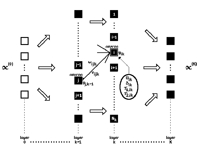

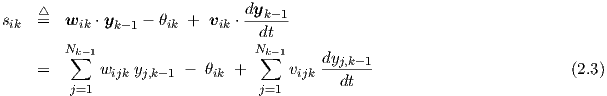
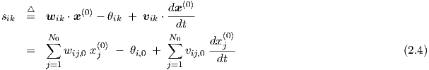
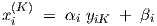
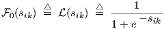
![△ 1--[ ( sik +-δik) ( sik---δik-)]
F1(sik,δik) = δ ln cosh 2 - ln cosh 2
ik s + δ
1-- cosh--ik2--ik-
= δik ln sik --δik (2.7)
cosh 2](thesis16x.png)
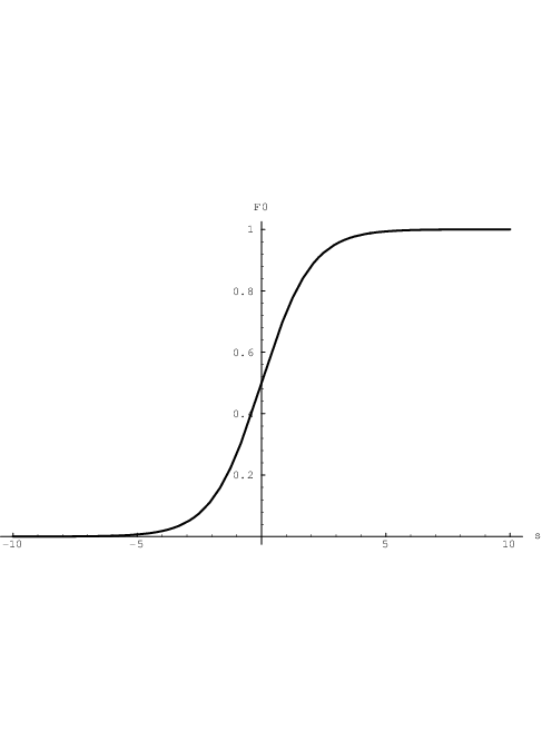
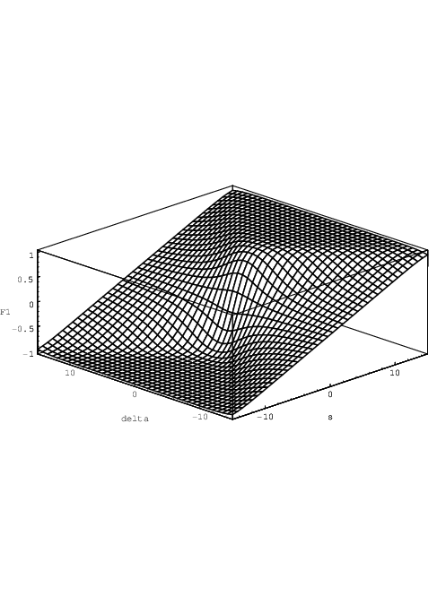
![△ 1 [ ( δ2 (s + 1)) ( δ2 (s - 1)) ]
F2(sik,δik) = -2- ln cosh-ik--ik----- - ln cosh -ik-ik-----
δik 2 2
δ2ik(sik +-1)
= 1--ln cosh------2----- (2.16)
δ2ik δ2ik(sik --1)
cosh 2](thesis25x.png)
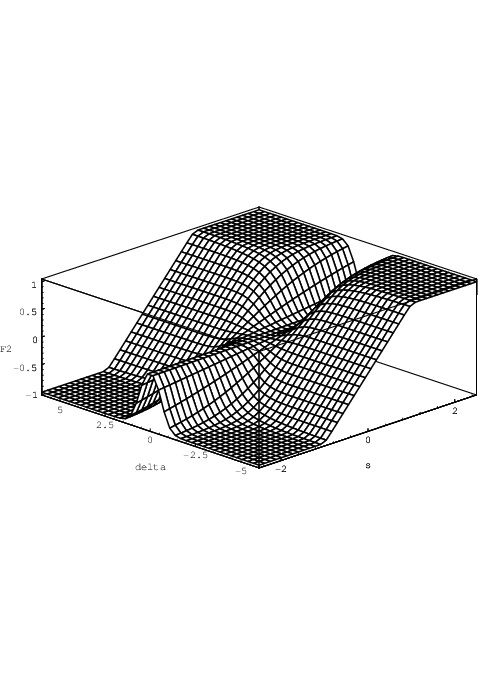
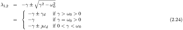
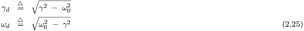

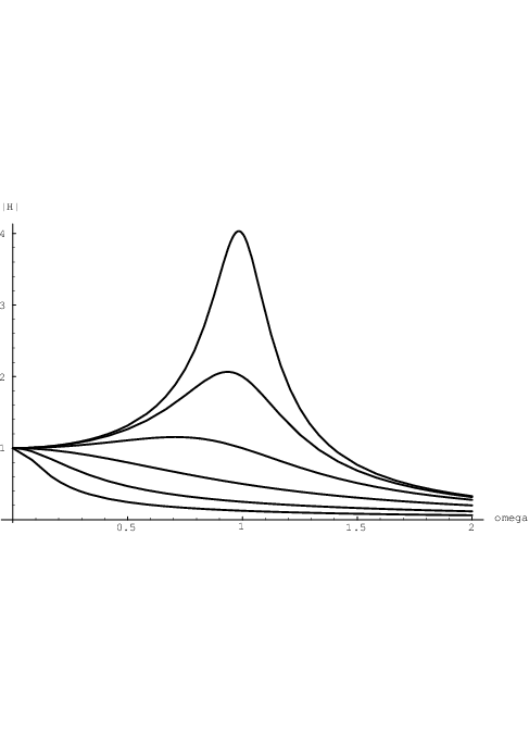
 for
for 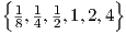 .
.
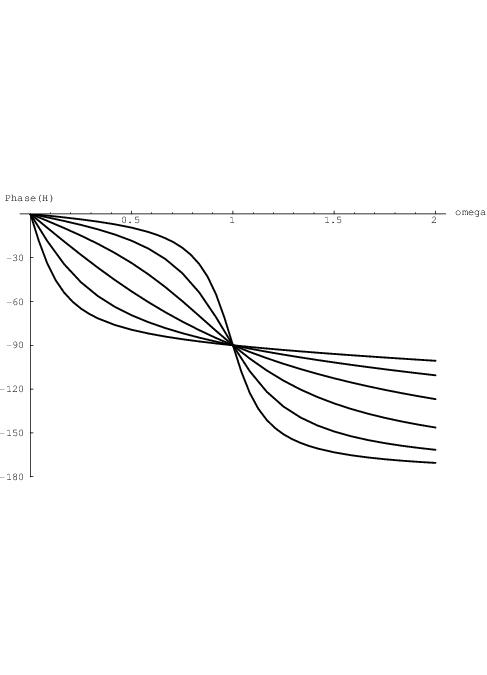

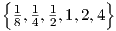 .
.

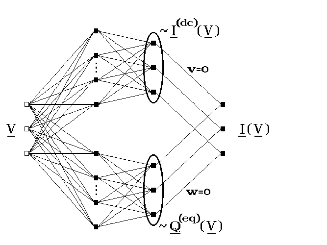
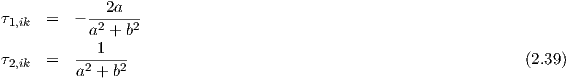
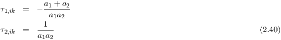
![( [ ( )] [ ( )] )
Vt c1 Is eV1∕Vt - 1 + c2 Is eV2∕Vt - 1
δ2- F2(sik,δik) ≡ Vt ln ( ------------------I------------------- + 1)
ik [ ( )] s [ ( )]
( c I eV1∕Vt - 1 + c I eV2∕Vt - 1 )
- Vt ln ( -2--s----------------1--s------------- + 1) (2.56)
Is](thesis101x.png)