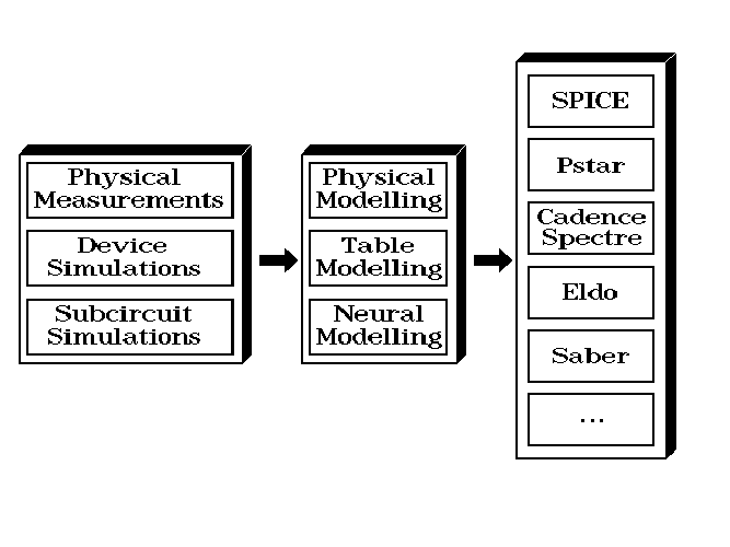
Figure 1.1:
Modelling for circuit simulation.
When dealing with semiconductor circuits and devices, one typically deals with continuous, but highly nonlinear, multidimensional dynamic systems. This makes it a difficult topic, and much scientific research is needed to improve the accuracy and efficiency with which the behaviour of these complicated analogue systems can be analyzed and predicted, i.e., simulated. New capabilities have to be developed to master the growing complexity in both analogue and digital design.
Very often, device-level simulation is simply too slow for simulating a (sub)circuit of any relevant size, while logic-level or switch-level simulation is considered too inaccurate for the critical circuit parts, while it is obviously limited to digital-type circuits only. The analogue circuit simulator often fills the gap by providing good analogue accuracy at a reasonable computational cost. Naturally, there is a continuous push both to improve the accuracy obtained from analogue circuit simulation, as well as to increase the capabilities for simulating very large circuits, containing many thousands of devices. These are to a large extent conflicting requirements, because higher accuracy tends to require more complicated models for the circuit components, while higher simulation speed favours the selection of simplified, but less accurate, models. The latter holds despite the general speed increase of available computer hardware on which one can run the circuit simulation software.
Apart from the important role of good models for devices and subcircuits, it is also very important to develop more powerful algorithms for solving the large systems of nonlinear equations that correspond to electronic circuits. However, in this thesis we will focus our attention on the development of device and subcircuit models, and in particular on possibilities to automate model development.
In the following sections, several approaches are outlined that aim at the generation of device and subcircuit models for use in analogue circuit simulators like Berkeley SPICE, Philips’ Pstar, Cadence Spectre, Anacad’s Eldo or Analogy’s Saber. A much simplified overview is shown in Fig. 1.1. Generally starting from discrete behavioural data1, the main objective is to arrive at continuous models that accurately match the discrete data, and that fulfill a number of additional requirements to make them suitable for use in circuit simulators.
In modelling for circuit simulation, there are two major applications that need to be distinguished because of their different requirements. The first modelling application is to develop efficient and sufficiently accurate device models for devices for which no model is available yet. The second application is to develop more efficient and still sufficiently accurate replacement models for subcircuits for which a detailed (network) “model” is often already available, namely as a description in terms of a set of interconnected transistors and other devices for which models are already available. Such efficient subcircuit replacement models are often called macromodels.
In the first application, the emphasis is often less on model efficiency and more on having something to do accurate circuit-level simulations with. Crudely stated: any model is better than no model. This holds in particular for technological advancements leading to new or significantly modified semiconductor devices. Then one will quickly want to know how circuits containing these devices will perform. At that stage, it is not yet crucial to have the efficiency provided by existing physical models for other devices—as long as the differences do not amount to orders of magnitude2. The latter condition usually excludes a direct interface between a circuit simulator and a device simulator, since the finite-element approach for a single device in a device simulator typically leads to thousands of nonlinear equations that have to be solved, thereby making it impractical to simulate circuits having more than a few transistors.
In the second application, the emphasis is on increasing efficiency without sacrificing too much accuracy w.r.t. a complete subcircuit description in terms of its constituent components. The latter is often possible, because designers strive to create near-ideal, e.g., near-linear, behaviour using devices that are themselves far from ideal. For example, a good linear amplifier may be built from many highly nonlinear bipolar transistors (for the gain) and linear resistors (for the linearity). Special circuitry may in addition be needed to obtain a good common mode rejection, a high bandwidth, a high slew rate, low offset currents, etc. In other words, designing for seemingly “simple” near-ideal behaviour usually requires a complicated circuit, but the macromodel for circuit simulation may be simple again, thereby gaining much in simulation efficiency.
At the device level, it is often possible to obtain discrete behavioural data from measurements and/or device simulations. One may think of a data set containing a list of applied voltages and corresponding device currents, but the list could also involve combinations of fluxes, charges, voltages and currents. Similarly, at the subcircuit level, one obtains such discrete behavioural data from measurements and/or (sub)circuit simulations. For analogue circuit simulation, however, a representation of electrical behaviour is needed that can in principle provide an outcome for any combination of input values, or bias conditions, where the input variables are usually a set of independent voltages, spanning a continuous real-valued input space IRn in case of n independent voltages. Consequently, something must be done to circumvent the discrete nature of the data in a data set.
The general approach is to develop a model that not only closely matches the behaviour as specified in the data set, but also yields “reasonable” outcomes for situations not specified in the data set. The vague notion of reasonable outcomes refers to several aspects. For situations that are close—according to some distance measure—to a situation from the data set, the model outcomes should also be close to the corresponding outcomes for that particular situation from the data set. Continuity of a model already implies this property to some extent, but strictly speaking only for infinitesimal distances. We wouldn’t be satisfied with a continuous but wildly oscillating interpolating model function. Therefore, the notion of reasonable outcomes also refers to certain constraints on the number of sign changes in higher derivatives of a model, by relating them to the number of sign changes in finite differences calculated from the data set3. Much more can be said about this topic, but for our purposes it should be sufficient to give some idea of what we mean by reasonable behaviour.
A model developed for use in a circuit simulator normally consists of a set of analytical functions that together define the model on its continuous input space IRn. For numerical and other reasons, the combination of functions that constitutes a model should be “smooth,” meaning that the model and its first—and preferably also higher—partial derivatives are continuous in the input variables. Furthermore, to incorporate effects like signal propagation delay, a device model may be constructed from several so-called quasistatic (sub)models.
A quasistatic model consists of functions describing the static behaviour, supplemented by functions of which the first time derivative is added to the outcomes of the static output functions to give a first order approximation of the effects of the rate with which input signals change. For example, a quasistatic MOSFET model normally contains nonlinear multidimensional functions—of the applied voltages—for the static (dc) terminal currents and also nonlinear multidimensional functions for equivalent terminal charges [48]; more details will be given in section 2.4.1. Time derivatives of the equivalent terminal charges form the capacitive currents. Time is not an explicit variable in any of these model functions: it only affects the model behaviour via the time dependence of the input variables of the model functions. Time may therefore only be explicitly present in the boundary conditions. This is entirely analogous to the fact that time is not an explicit variable in, for instance, the laws of Newtonian mechanics or the Maxwell equations, while actual physical problems in those areas are solved by imposing an explicit time dependence in the boundary conditions. True delays inside quasistatic models do not exist, because the behaviour of a quasistatic model is directly and instantaneously determined by the behaviour of its input variables4. In other words, a quasistatic model has no internal state variables (memory variables) that could affect its behaviour. Any charge storage is only associated with the terminals of the quasistatic model.
The Kirchhoff current law (KCL) relates the behaviour of different topologically neighbouring quasistatic models, by requiring that the sum of the terminal currents flowing towards a shared circuit node should be zero in order to conserve charge [10]. It is through the corresponding differential algebraic equations (DAE’s) that truly dynamic effects like delays are accounted for. Non-input, non-output circuit nodes are called internal nodes, and a model or circuit containing internal nodes can represent truly dynamic or non-quasistatic behaviour, because the charge associated with an internal node acts as an internal state (memory) variable.
A non-quasistatic model is simply a model that can—via the internal nodes—represent the non-instantaneous responses that quasistatic models cannot capture by themselves. A set of interconnected quasistatic models then constitutes a non-quasistatic model through the KCL equations. Essentially, a non-quasistatic model may be viewed as a small circuit by itself, but the internal structure of this circuit need no longer correspond to the physical structure of the device or subcircuit that it represents, because the main purpose of the non-quasistatic model may be to accurately represent the electrical behaviour, not the underlying physical structure.
The classical approach to obtain a suitable compact model for circuit simulation has been to make use of available physical knowledge, and to forge that knowledge into a numerically well-behaved model. A monograph on physical MOSFET modelling is for instance [48]. The Philips’ MOST model 9 and bipolar model MEXTRAM are examples of advanced physical models [21]. The relation with the underlying device physics and physical structure remains a very important asset of such hand-crafted models. On the other hand, a major disadvantage of physical modelling is that it usually takes years to develop a good model for a new device. That has been one of the major reasons to explore alternative modelling techniques.
Because of many complications in developing a physical model, the resulting model often contains several constructions that are more of a curve-fitting nature instead of being based on physics. This is common in cases where analytical expressions can be derived only for idealized asymptotic behaviour occurring deep within distinct operating regions. Transition regions in multidimensional behaviour are then simply—but certainly not easily—modelled by carefully designed transition functions for the desired intermediate behaviour. Consequently, advanced physical models are in practice at least partly phenomenological models in order to meet the accuracy and smoothness requirements. Apparently, the phenomenological approach offers some advantages when pure physical modelling runs into trouble, and it is therefore logical and legitimate to ask whether a purely phenomenological approach would be feasible and worthwhile. Phenomenological modelling in its extreme form is a kind of black-box modelling, giving an accurate representation of behaviour without knowing anything about the causes of that behaviour.
Apart from using physical knowledge to derive or build a model, one could also apply numerical interpolation or approximation of discrete data. The merits of this kind of black-box approach, and a number of useful techniques, are described in detail in [11, 38, 39]. The models resulting from these techniques are called table models. A very important advantage of table modelling techniques is that one can in principle obtain a quasistatic model of any required accuracy by providing a sufficient amount of (sufficiently accurate) discrete data. Optimization techniques are not necessary—although optimization can be employed to further improve the accuracy. Table modelling can be applied without the risk of finding a poor fit due to some local minimum resulting from optimization. However, a major disadvantage is that a single quasistatic model cannot express all kinds of behaviour relevant to device and subcircuit modelling.
Table modelling has so far been restricted to the generation of a single quasistatic model of the whole device or subcircuit to be modelled, thereby neglecting the consequences of non-instantaneous response. Furthermore, for rather fundamental reasons, it is not possible to obtain even low-dimensional interpolating table models that are both infinitely smooth (infinitely differentiable, i.e., C∞) and computationally efficient5. In addition, the computational cost of evaluating the table models for a given input grows exponentially with the number of input variables, because knowledge about the underlying physical structure of the device is not exploited in order to reduce the number of relevant terms that contain multidimensional combinations of input variables6.
Hybrid modelling approaches have been tried for specific devices, but this again increases the time needed to model new devices, because of the re-introduction of rather device-specific physical knowledge. For instance, in MOSFET modelling one could apply separate—nested—table models for modelling the dependence of the threshold voltage on voltage bias, and for the dependence of dc current on threshold and voltage bias. Clearly, apart from any further choices to reduce the dimensionality of the table models, the introduction of a threshold variable as an intermediate, and distinguishable, entity already makes this approach rather device-specific.
In recent years, much attention has been paid in applying artificial neural networks to learn to represent mappings of different sorts. In this thesis, we investigate the possibility of designing artificial neural networks in such a way, that they will be able to learn to represent the static and dynamic behaviour of electronic devices and (sub)circuits. Learning here refers to optimization of the degree to which some desired behaviour, the target behaviour, is represented. The terms learning and optimization are therefore nowadays often used interchangeably, although the term learning is normally used only in conjunction with (artificial) neural networks, because, historically, learning used to refer to behavioural changes occurring through—synaptic and other—adaptations within biological neural networks. The analogy with biology, and its terminology, is simply stretched when dealing with artificial systems that bear a remote resemblance to biological neural networks.
As was explained before, in order to model the behavioural consequences of delays within devices or subcircuits, non-quasistatic (dynamic) modelling is required. This implies the use of internal nodes with their associated state variables for (leaky) memory. For numerical reasons, in particular during time domain analysis in a circuit simulator, models should not only be accurate, but also “smooth,” implying at least continuity of the model and its first partial derivatives. In order to deal with higher harmonics in distortion analyses, higher-order derivatives must also be continuous, which is very difficult or costly to obtain both with table modelling and with conventional physical device modelling.
Furthermore, contrary to the practical situation with table modelling, the best internal coordinate system for modelling should preferably arise automatically, while fewer restrictions on the specification of measurements for device simulations for model input would be quite welcome to the user: a grid-free approach would make the usage of automatic modelling methods easier, ideally implying not much more than providing measurement data to the automatic modelling procedure, only ensuring that the selected data set sufficiently characterizes (“covers”) the device behaviour. Finally, better guarantees for monotonicity, wherever applicable, can also be advantageous, for example in avoiding artefacts in simulated circuit behaviour.
Clearly, this list of requirements for an automatic non-quasistatic modelling scheme is ambitious, but the situation is not entirely hopeless. As it turns out, a number of ideas derived from contemporary advances in neural network theory, in particular the backpropagation theory (also called the “generalized delta rule”) for feedforward networks, together with our recent work on device modelling and circuit simulation, can be merged into a new and probably viable modelling strategy, the foundations of which are assembled in the following chapters.
From the recent literature, one may even anticipate that the mainstreams of electronic circuit theory and neural network theory will in forthcoming decades converge into general methodologies for the optimization of analogue nonlinear dynamic systems. As a demonstration of the viability of such a merger, a new modelling method will be described, which combines and extends ideas borrowed from methods and applications in electronic circuit and device modelling theory and numerical analysis [8, 9, 10, 29, 37, 39], the popular error backpropagation method (and other methods) for neural networks [1, 2, 18, 22, 36, 44, 51], and time domain extensions to neural networks in order to deal with dynamic systems [5, 25, 28, 40, 42, 45, 47, 49, 50]. The two most prevalent approaches extend either the fully connected—except for the often zero-valued self-connections—Hopfield-type networks, or the feedforward networks used in backpropagation learning. We will basically describe extensions along this second line, because the absence of feedback loops greatly facilitates giving theoretical guarantees on several desirable model(ling) properties.
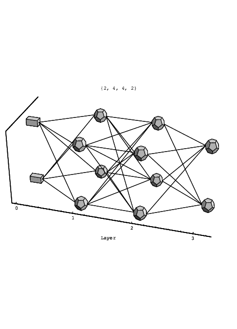
An example of a layered feedforward network is shown in the 3D plot of Fig. 1.2. This kind of network is sometimes also called a multilayer perceptron (MLP) network. Connections only exist between neurons in subsequent layers: subsequent neuron layers are fully interconnected, but connections among neurons within a layer do not exist, nor are there any direct connections across layers. This is the kind of network topology that will be discussed in this thesis, and it can be easily characterized by the number of neurons in each layer, going from input layer (layer 0) to output layer: in Fig. 1.2, the network has a 2-4-4-2 topology7, where the network inputs are enforced upon the two rectangular input nodes shown at the left side. The actual neural processing elements are denoted by dodecahedrons, such that this particular network contains 10 neurons8. The network in Fig. 1.2 has two so-called hidden layers, meaning the non-input, non-output layers, i.e., layer 1 and 2. The signals in a feedforward neural network propagate from one network layer to the next. The signal flow is unidirectional: the input to a neuron depends only on the outputs of neurons in the preceding layer, such that no feedback loops exist in the network9.
We will consider the network of Fig. 1.2 to be a 4-layer network, thus including the layer of network inputs in counting layers. There is no general agreement in the literature on whether or not to count the input layer, because it does not compute anything. Therefore, one might prefer to call the network of Fig. 1.2 a 3-layer network. On the other hand, the input layer clearly is a layer, and the number of neural connections to the next layer grows linearly with the number of network inputs, which makes it convenient to consider the input layer as part of the neural network. Therefore one should notice that, although in this thesis the input layer is considered as part of the neural network, a different convention or interpretation will be found in some of the referenced literature. In many cases we will try to circumvent this potential source of confusion by specifying the number of hidden layers of a neural network, instead of specifying the total number of layers.
In this thesis, the number of layers in a feedforward neural network is arbitrary, although more than two hidden layers are in practice not often used. The number of neurons in each layer is also arbitrary. The preferred number of layers, as well as the preferred number of neurons in each of the hidden layers, is usually determined via educated guesses and some trial and error on the problem at hand, to find the simplest network that gives acceptable performance.
Some researchers create time domain extensions to neural networks via schemes that can be loosely described as being tapped delay lines (the ARMA model used in adaptive filtering also belongs to this class), as in, e.g., [41]. That discrete-time approach essentially concerns ways to evaluate discretized and truncated convolution integrals. In our continuous-time application, we wish to avoid any explicit time discretization in the (finally resulting) model description, because we later want to obtain a description in terms of—continuous-time—differential equations. These differential equations can then be mapped onto equivalent representations that are suitable for use in a circuit simulator, which generally contains sophisticated methods for automatically selecting appropriate time step sizes and integration orders. In other words, we should determine the coefficients of a set of differential equations rather than parameters like delays and tapping weights that have a discrete-time nature or are associated with a particular pre-selected time discretization. In order to determine the coefficients of a set of differential equations, we will in fact need a temporary discretization to make the analysis tractable, but that discretization is not in any way part of the final result, the neural model.
The following list summarizes and discusses some of the potential benefits that may ideally be obtained from the new neural modelling approach—what can be achieved in practice with dynamic neural networks remains to be seen. However, a few of the potential benefits have already been turned into facts, as will be shown in subsequent sections. It should be noted, that the list of potential benefits may be shared, at least in part, by other black-box modelling techniques.
An efficient link, via neural network models, between device simulation and circuit simulation allows for the anticipation of consequences of technological choices to circuit performance. This may result in early shifts in device design, processing efforts and circuit design, as it can take place ahead of actual manufacturing capabilities: the device need not (yet) physically exist. Neural network models could then contribute to a reduction of the time-to-market of circuit designs using promising new semiconductor device technologies.
Even though the underlying physics cannot be traced within the black-box neural models, the link with physics can still be preserved if the target data is generated by a device simulator, because one can perform additional device simulations to find out how, for instance, diffusion profiles affect the device characteristics. Then one can change the (simulated or real) processing steps accordingly, and have the neural networks adapt to the modified characteristics, after which one can study the effects on circuit-level simulations.
Not only the ever decreasing characteristic feature sizes in VLSI technology cause multidimensional interactions that are hard to analyze physically and mathematically, but also the ever higher frequencies at which these smaller devices are operated cause multidimensional interactions, which in turn lead to major physical and mathematical modelling difficulties. This happens not only at the VLSI level. For instance, parasitic inductances and capacitances due to packaging technology become nonnegligible at very high frequencies. For discrete bipolar devices, this is already a serious problem in practical applications.
At some stage, the physical model, even if one can be derived, may become so detailed—i.e., contain so much structural information about the device—that the border between device simulation and circuit simulation becomes blurred, at the expense of simulation efficiency. Although the mathematics becomes more difficult and elaborate when more physical high-frequency interactions are incorporated in the analysis, the actual behaviour of the device or subcircuit does not necessarily become more complicated. Different physical causes may have similar behavioural effects, or partly counteract each other, such that a simple(r) equivalent behavioural model may still exist11.
Neural modelling is not hampered by any complicated causes of behaviour: it just concerns the accurate representation of behaviour, in a form that is suitable for its main application area, which in our case is analogue circuit simulation.
Model smoothness is also important for the efficiency of the higher order time integration schemes of an analogue circuit simulator. The time integration routines in a circuit simulator typically detect discontinuities of orders that are less than the integration order being used, and respond by temporarily lowering the integration order and/or time step size, which causes significant computational overhead during transient simulations.
The monotonicity guarantee for neural networks can be maintained for highly nonlinear multidimensional behaviour, which so far has not been possible with table models without requiring excessive amounts of data [39]. Furthermore, the monotonicity guarantee is optional, such that nonmonotonic static behaviour can still be modelled, as is illustrated in section 4.2.1.
On the other hand, it is at the same time a limitation to the modelling capabilities of these neural networks, for there may be situations in which one wants to model the multiple solutions in the behaviour of a resistive device or subcircuit, for example when modelling a flip-flop. So it must be a deliberate choice, made to help with the modelling of a restricted class of devices and subcircuits. In this thesis, the uniqueness restriction is accepted in order to make use of the associated desirable mathematical and numerical properties.
The general heading of this thesis is to first define a class of dynamic neural networks, then to derive a theory and algorithms for training these neural networks, subsequently to implement the theory and algorithms in software, and then to apply the software to a number of test-cases. Of course, this idealized logical structure does not quite reflect the way the work is done, in view of the complexity of the subject. In reality one has to consider, as early as possible, aspects from all these stages at the same time, in order to increase the probability of obtaining a practical compromise between the many conflicting requirements. Moreover, insights gained from software experiments may in a sense “backpropagate” and lead to changes even in the neural network definitions.
In chapter 2, the equations for dynamic feedforward neural networks are defined and discussed. The behaviour of individual neurons is analyzed in detail. In addition, the representational capabilities of these networks are considered, as well as some possibilities to construct equivalent electrical circuits for neurons, thereby allowing their direct application in analogue circuit simulators.
Chapter 3 shows how the definitions of chapter 2 can be used to construct sensitivity-based learning procedures for dynamic feedforward neural networks. The chapter has two major parts, consisting of sections 3.1 and 3.2. Section 3.1 considers a representation in the time domain, in which neural networks may have to learn step responses or other transient responses. Section 3.2 shows how the definitions of chapter 2 can also be employed in a small-signal frequency domain representation, by deriving a corresponding sensitivity-based learning approach for the frequency domain. Time domain learning can subsequently be combined with frequency domain learning. As a special topic, section 3.3 discusses how monotonicity of the static response of feedforward neural networks can be guaranteed via parameter constraints during learning. The monotonicity property is particularly important for the development of suitable device models for use in analogue circuit simulators.
Chapter 4, section 4.1, discusses several aspects concerning an experimental software implementation of the time domain learning and frequency domain learning techniques of the preceding chapter. Section 4.2 then shows a number of preliminary modelling results obtained with this experimental software implementation. The neural modelling examples involve time domain learning and frequency domain learning, and use is made of the possibility to automatically generate analogue behavioural (macro)models for circuit simulators.
Finally, chapter 5 draws some general conclusions and sketches recommended directions for further research.