Chapter 4
Results

4.1 Experimental Software

This chapter describes some aspects of an ANSI C software implementation of the learning methods as described in the preceding chapters. The experimental software implementation, presently measuring some 25000 lines of source code, runs on Apollo/HP425T workstations using GPR graphics, on PC’s using MS-Windows 95 and on HP9000/735 systems using XWindows graphics. The software is capable of simultaneously simulating and optimizing an arbitrary number of dynamic feedforward neural networks in time and frequency domain. These neural networks can have any number of inputs and outputs, and any number of layers.

4.1.1 On the Use of Scaling Techniques

Scaling is used to make optimization insensitive to units of training data, by applying a linear transformation—often just an inner product with a vector of scaling factors—to the inputs and outputs of the network, the internal network parameters and the training data. By using scaling, it no longer makes any difference to the software whether, say, input voltages were specified in megavolts or millivolts, or output currents in kiloampères or microampères.

Some optimization techniques are invariant to scaling, but many of them—e.g., steepest descent—are not. Therefore, the safest way to deal in general with this potential hazard is to always scale the network inputs and outputs to a preferred range: one then no longer needs to bother whether an optimization technique is entirely scale invariant (including its heuristic extensions and adaptations). Because this scaling only involves a simple pre- and postprocessing, the computational overhead is generally negligible. Scaling, to bring numbers closer to 1, also helps to prevent or alleviate additional numerical problems like the loss of significant digits, as well as floating point underflow and overflow.

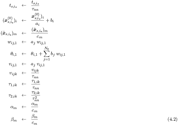
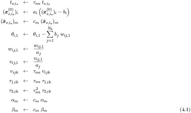
For dc and transient, the following scaling and unscaling rules apply to the i-th network input and the m-th network output:

• A multiplicative scaling a_i, during preprocessing, of the network input values in the training data, is undone in the postprocessing (after optimization) by multiplying the weight parameters w_ij,1 and v_ij,1 (i.e., only in network layer k = 1) by this same network input value data scaling factor. Essentially, one afterwards increases the sensitivity of the network input stage with the same measure by which the training input values had been artificially amplified before training was started.
• Similarly, a multiplicative scaling c_m of the network target output values, also performed during preprocessing, is undone in the postprocessing by dividing the α_m- and β_m-values for the network output layer by the target data scaling factor used in the preprocessing.
• The scaling of transient time points by a factor τ_nn, during preprocessing, is undone in the postprocessing by dividing the v_ijk- and τ_1,ik-values of all neurons by the time points scaling factor τ_nn used in the preprocessing. All τ_2,ik-values are divided by the square of this factor, because they are the coefficients of the second derivative w.r.t. time in the neuron differential equations of the form (2.2).
• A translation scaling by an amount b_i may be applied to shift the input data to positions near the origin.

If we use for the network input i an input shift -b_i, followed by a multiplicative scaling a_i, and if we use a multiplicative scaling c_m for network output m, and apply a time scaling τ_nn, we can write the scaling of training data and network parameters as

The treatment of ac scaling runs along rather similar lines, by translating the ac scalings into their corresponding time domain scalings, and vice versa. The inverse of a frequency scaling is in fact a time scaling. The scaling of ac frequency points, during preprocessing, is therefore also undone in the postprocessing by dividing the v_ijk- and τ_1,ik-values of all neurons by this corresponding time scaling factor τ_nn, determined and used in the preprocessing. Again, all τ_2,ik-values are divided by the square of this time scaling factor.

The scaling of target transfer matrix elements refers to phasor ratio’s of network target outputs and network inputs. Multiplying all the w_ij,1 and v_ij,1 by a single constant would not affect the elements of the neural network transfer matrices if all the α_m and β_m were divided by that same constant. Therefore, a separate network input and target output scaling cannot be uniquely determined, but may simply be taken from the dc and transient training data. Hence, these transfer matrix elements are during pre-processing scaled by the target scaling factor divided by the input scaling factor, as determined for dc and transient. For multiple-input-multiple-output networks, this implies the use of a scaling matrix with elements coming from all possible combinations of network inputs and network outputs.

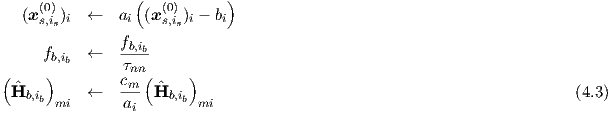
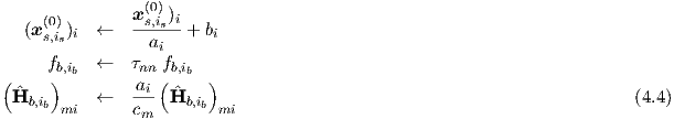
The scaling of frequency domain data for dc bias conditions x_s,is⁽⁰⁾ can therefore be written as

This discussion on scaling is certainly not complete, since one can also apply scaling to, for instance, the error functions, while such a scaling may in principle be different for each network output item. It would lead too far, however, to go into all the intricacies and pitfalls of input and output scaling for nonlinear dynamic systems. Many of these matters are presently still under investigation, because they can have a profound effect on the learning performance.

4.1.2 Nonlinear Constraints on Dynamic Behaviour

Although the neural modelling techniques form a kind of black-box approach, inclusion of general a priori knowledge about the field of application in the form of parameter constraints can increase the performance of optimization techniques in several respects. It may lead to fewer optimization iterations, and it may reduce the probability of getting stuck at a local minimum with a poor fit to the target data. On the other hand, constraints should not be too strict, but rather “encourage” the optimization techniques to find what we consider “reasonable” network behaviour, by making it more difficult to obtain “exotic” behaviour.

Figure 4.1:

Parameter function τ₁(σ_1,ik , σ_2,ik) for Q_max = 1 and c_d = 1.

Figure 4.2:

Parameter function τ₂(σ_1,ik , σ_2,ik) for Q_max = 1 and c_d = 1.

The neuron timing parameters τ_1,ik and τ_2,ik should remain non-negative, such that the neural network outcomes will not, for instance, continue to grow indefinitely with time. If there are good reasons to assume that a device will not behave as a near-resonant circuit, the value of the neuron quality factors may be bounded by means of constraints. Without such constraints, a neural network may try to approximate, i.e., learn, the behaviour corresponding to a band-pass filter characteristic by first growing large but narrow resonance peaks¹. This can quickly yield a crude approximation with peaks at the right positions, but resonant behaviour is qualitatively different from the behaviour of a band-pass filter, where the height and width of a peak in the frequency transfer curve can be set independently by an appropriate choice of parameters. Resonant behaviour corresponds to small τ_1,ik values, but band-pass filter behaviour corresponds to the subsequent dominance, with growing frequency, of terms involving v_ijk, τ_1,ik and τ_2,ik, respectively. This means that a first quick approximation with resonance peaks must subsequently be “unlearned” to find a band-pass type of representation, at the expense of additional optimization iterations—if the neural network is not in the mean time already caught at a local minimum of the error function.

It is worth noting that the computational burden of calculating τ’s from σ’s and σ’s from τ’s, is generally negligible even for rather complicated transformations. The reason is, that the actual ac, dc and transient sensitivity calculations can, for the whole training set, be based on using only the τ’s instead of the σ’s. The τ’s and σ’s need to be updated only once per optimization iteration, and the required sensitivity information w.r.t. the σ’s is only at that instant calculated via evaluation of the partial derivatives of the parameter functions τ₁(σ_1,ik,σ_2,ik) and τ₂(σ_1,ik,σ_2,ik).

4.1.2.1 Scheme for τ_1,ik,τ_2,ik > 0 and bounded τ_1,ik

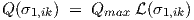
The timing parameter τ_2,ik can be expressed in terms of τ_1,ik and the quality factor Q by rewriting Eq. (2.22) as τ_2,ik = (τ_1,ik Q)², while a bounded Q may be obtained by multiplying a default, or user-specified, maximum quality factor Q_max by the logistic function (σ_1,ik) as in

(4.5)

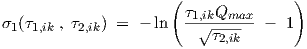
such that 0 < Q(σ_1,ik) < Q_max for all real-valued σ_1,ik. When using an initial value σ_1,ik = 0, this would correspond to an initial quality factor Q = Q_max .

Another point to be considered, is what kind of behaviour we expect at the frequency corresponding to the time scaling by τ_nn. This time scaling should be chosen in such a way, that the major time constants of the neural network come into play at a scaled frequency ω_s ≈ 1. Also, the network scaling should preferably be such, that a good approximation to the target data is obtained with many of the scaled parameter values in the neighbourhood of 1. Furthermore, for these parameter values, and at ω_s, the “typical” influence of the parameters on the network behaviour should neither be completely negligible nor highly dominant. If they are too dominant, we apparently have a large number of other network parameters that do not play a significant role, which means that, during network evaluation, much computational effort is wasted on expressions that do not contribute much to accuracy. Vice versa, if their influence is negligible, computational effort is wasted on expressions containing these redundant parameters. The degrees of freedom provided by the network parameters are best exploited, when each network parameter plays a meaningful or significant role. Even if this ideal situation is never reached, it still is an important qualitative observation that can help to obtain a reasonably efficient neural model.

For ω = ω_s = 1, the denominator of the neuron transfer function in Eq. (3.35) equals 1 + ȷτ_1,ik - τ_2,ik . The dominance of the second and third term may, for this special frequency, be bounded by requiring that τ_1,ik + τ_2,ik < c_d, with c_d a positive real constant, having a default value that is not much larger than 1. Substitution of τ_2,ik = (τ_1,ik Q)², and allowing only positive τ_1,ik values, leads to the equivalent requirement 0 < τ_1,ik < 2c_d ∕ (1 + ). This requirement may be fulfilled by using the logistic function (σ_2,ik) in the following expression for the τ₁ parameter function

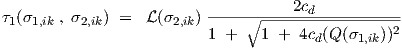
(4.6)

and τ_2,ik is then obtained from the τ₂ parameter function

(4.7)

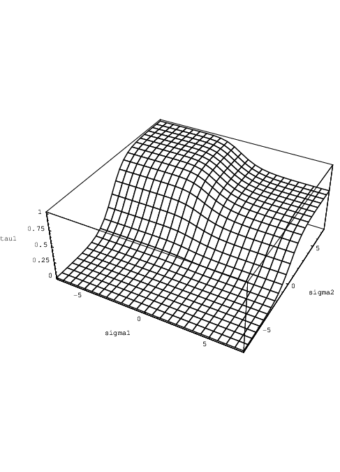
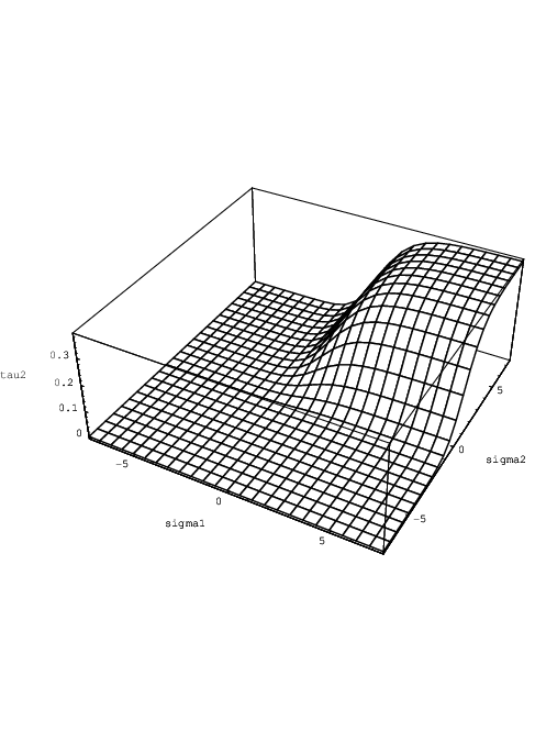
The shapes of the parameter functions τ₁(σ_1,ik , σ_2,ik) and τ₂(σ_1,ik , σ_2,ik) are illustrated in Figs. 4.1 and 4.2, using Q_max = 1 and c_d = 1.

We deliberately did not make use of the value of ω₀ , as defined in (2.21), to construct relevant constraints. For large values of the quality factor (Q ≫ 1), ω₀ would indeed be the angular frequency at which the denominator of the neuron transfer function in Eq. (3.35) starts to deviate significantly from 1, for values of τ_1,ik and τ_2,ik in the neighbourhood of 1, because the complex-valued term with τ_1,ik can in that case be neglected. This becomes immediately apparent if we rewrite the denominator from Eq. (3.35), using Eqs. (2.21) and (2.22), in the form 1 + ȷ(1∕Q)(ω∕ω₀) - (ω∕ω₀)². However, for small values of the quality factor (Q ≪ 1), the term with τ_1,ik in the denominator of Eq. (3.35) clearly becomes significant at angular frequencies lying far below ω₀—namely by a factor on the order of the quality factor Q.

Near-resonant behaviour is relatively uncommon for semiconductor devices at normal operating frequencies, although with high-frequency discrete devices it can occur due to the packaging. The inductance of bonding wires can, together with parasitic capacitances, form linear subcircuits with high quality factors. Usually, some a priori knowledge is available about the device or subcircuit to be modelled, thereby allowing an educated guess for Q_max. If one prescribes too small a value for Q_max, one will discover this—apart from a poor fit to the target data—specifically from the large values for σ₁ that arise from the optimization. When this happens, an effective and efficient countermeasure is to continue the optimization with a larger value of Q_max. The continuation can be done without disrupting the optimization results obtained thus far, by recalculating the σ values from the latest τ values, given the new—larger—value of Q_max. For this reason, the above parameter functions τ₁(σ_1,ik,σ_2,ik) and τ₂(σ_1,ik,σ_2,ik) were also designed to be explicitly invertible functions for values of τ_1,ik and τ_2,ik that meet the above constraints involving Q_max and c_d. This means that we can write down explicit expressions for σ_1,ik = σ₁(τ_1,ik,τ_2,ik) and σ_2,ik = σ₂(τ_1,ik,τ_2,ik). These expressions are given by

(4.8)

and

(4.9)

with Q calculated from Q = ∕τ_1,ik .

4.1.2.2 Alternative scheme for τ_1,ik,τ_2,ik ≥ 0

In some cases, particularly when modelling filter circuits, it may be difficult to find a suitable value for c_d. If c_d is not large enough, then obviously one may have put too severe restrictions to the behaviour of neurons. However, if it is too large, finding a correspondingly large negative σ_2,ik value may take many learning iterations. Similarly, using the logistic function to impose constraints may lead to many learning iterations when the range of time constants to be modelled is large. For reasons like these, the following simpler alternative scheme can be used instead:

(4.10)

(4.11)

with

(4.12)

and σ_1,ik and σ_2,ik values can be recalculated from proper τ_1,ik and τ_2,ik values using

(4.13)

(4.14)

4.1.3 Software Self-Test Mode

An important aspect in program development is the correctness of the software. In the software engineering discipline, some people advocate the use of formal techniques for proving program correctness. However, formal techniques for proving program correctness have not yet been demonstrated to be applicable to complicated engineering packages, and it seems unlikely that these techniques will play such a role in the foreseeable future².

Figure 4.3:

Program running in sensitivity self-test mode.

It is hard to prove that a proof of program correctness is itself correct, especially if the proof is much longer and harder to read than the program one wishes to verify. It is also very difficult to make sure that the specification of software functionality is correct. One could have a “correct” program that perfectly meets a nonsensical specification. Essentially, one could even view the source code of a program as a (very detailed) specification of its desired functionality, since there is no fundamental distinction between a software specification and a detailed software design or a computer program. In fact, there is only the practical convention that by definition a software specification is mapped onto a software design, and a software design is mapped onto a computer program, while adding detail (also to be verified) in each mapping: a kind of divide-and-conquer approach.

What one can do, however, is to try several methodologically and/or algorithmically very distinct routes to the solution of given test problems. To be more concrete: one can in simple cases derive solutions mathematically, and test whether the software gives the same solutions in these trial cases.

In addition, and directly applicable to our experimental software, one can check whether analytically derived expressions for sensitivity give, within an estimated accuracy range, the same outcomes as numerical (approximations of) derivatives via finite difference expressions. The latter are far more easy to derive and program, but also far more inefficient to calculate. During network optimization, one would for efficiency use only the analytical sensitivity calculations. However, because dc, transient and ac sensitivity form the core of the neural network learning program, the calculation of both analytical and numerical derivatives has been implemented as a self-test mode with graphical output, such that one can verify the correctness of sensitivity calculations for each individual parameter in turn in a set of neural networks, and for a large number of time points and frequency points.

In Fig. 4.3 a hardcopy of the Apollo/HP425T screen shows the graphical output while running in the self-test mode. On the left side, in the first column of the graphics matrix, the topologies for three different feedforward neural networks are shown. Associated transient sensitivity and ac sensitivity curves are shown in the second and third column, respectively. The neuron for which the sensitivity w.r.t. one particular parameter is being calculated, is highlighted by a surrounding small rectangle—in Fig. 4.3 the top left neuron of network NET2. It must be emphasized, that the drawn sensitivity curves show the “momentary” sensitivity contributions, not the accumulated total sensitivity up to a given time or frequency point. This means that in the self-test mode the summations in Eqs. (3.20) and (3.61), and in the corresponding gradients in Eqs. (3.25) and (3.64), are actually suppressed in order to reduce numerical masking of any potential errors in the implementation of sensitivity calculations. However, for transient sensitivity, the dependence of sensitivity values (“sensitivity state”) on preceding time points is still taken into account, because it is very important to also check the correctness of this dependence as specified in Eq. (3.8).

The curves for analytical and numerical sensitivity completely coincide in Fig. 4.3, indicating that an error in these calculations is unlikely. The program cycles through the sensitivity curves for all network parameters, so the hardcopy shows only a small fraction of the output of a self-test run. Because the self-test option has been made an integral part of the program, correctness can without effort be quickly re-checked at any moment, e.g., after a change in implementation: one just watches for any non-coinciding curves, which gives a very good fault coverage.

4.1.4 Graphical Output in Learning Mode

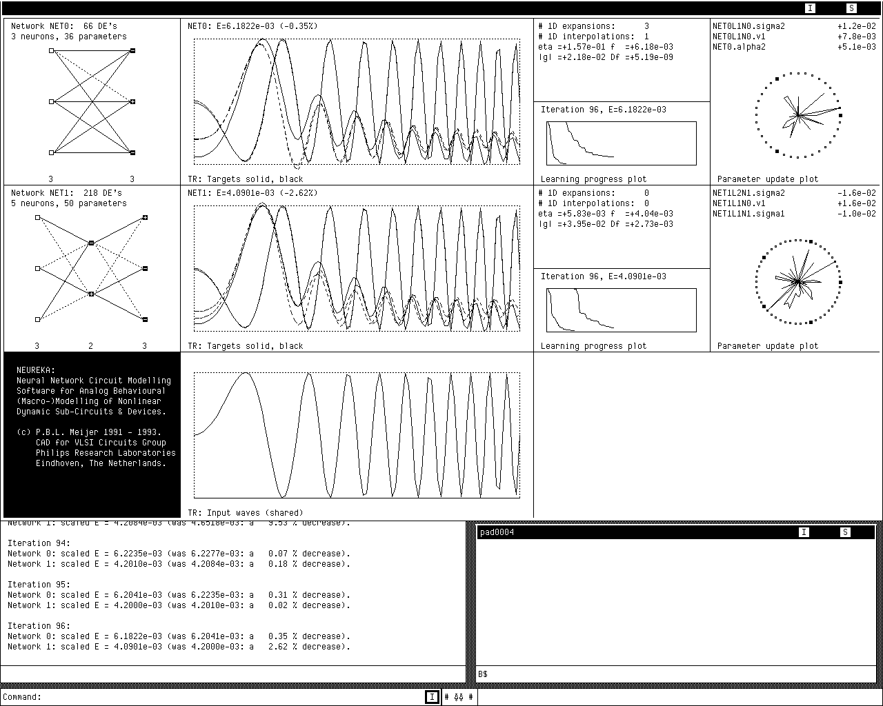
A hardcopy of the Apollo/HP425T screen, presented in Fig. 4.4, shows some typical graphical output as obtained during simultaneous time domain learning in multiple dynamic neural networks. Typically, one simulates and trains several slightly different neural network topologies in one run, in order to select afterwards the best compromise between simplicity (computational efficiency) of the generated models and their accuracy w.r.t. the training data.

Figure 4.4:

Program running in neural network learning mode.

In the hardcopy of Fig. 4.4, a single graphics window is subdivided to form a 3 × 4 graphics matrix showing information about the training of two neural networks.

On the left side, in the first column of the graphics matrix, the topologies for two different feedforward neural networks are shown. Associated time domain curves are shown in the second column. In the network plots, any positive network weights w_ijk are shown by solid interconnect lines, while dotted lines are used for negative weights³. A small plus or minus sign within a neuron i in layer k represents the sign of its associated threshold θ_ik. The network inputs are shown as dummy neurons, indicated by open squares, on the left side of the topology plots. The number of neurons within each layer is shown at the bottom of these plots. We will use the notational convention that the feedforward network topology can be characterized by a sequence of numbers, for the number of neurons in each layer, going from input (left in the plots) to the output (right). Consequently, NET1 in Fig. 4.4 is a 3-2-3 network: 3 inputs (dummy neurons), 2 neurons in the middle (hidden) layer, and 3 output neurons.

If there were also frequency domain data in the training set, the second column of the graphics matrix of Fig. 4.4 would be split into two columns with plots for both time domain and frequency domain results—in a similar fashion as shown before for the self-test mode in Fig. 4.3. The target data as a function of time is shown by solid curves, and the actual network behaviour, in this case obtained using Backward Euler time integration, is represented by dashed curves. At the bottom of the graphics window, the input waves are shown. All target curves are automatically and individually scaled to fit the subwindows, so the range and offset of different target curves may be very different even if they seem to have the same range on the screen. This helps to visualize the behavioural structure—e.g., peaks and valleys—in all of the curves, independent of differences in dynamic range, at the expense of the visualization of the relative ranges and offsets.

Small error plots in the third column of the graphics matrix (“Learning progress plot”) show the progress made in reducing the modelling error. If the error has dropped by more than a factor of a hundred, the vertical scale is automatically enlarged by this factor in order to show further learning progress. This causes the upward jumps in the plots.

The fourth column of the graphics matrix (“Parameter update plot”) contains information on the relative size of all parameter changes in each iteration, together with numerical values for the three largest absolute changes. The many dimensions in the network parameter vector are captured by a logarithmically compressed “smashed mosquito” plot, where each direction corresponds to a particular parameter, and where larger parameter changes yield points further away from the central point. The purpose of this kind of information is to give some insight into what is going on during the optimization of high-dimensional systems.

The target data were in this case obtained from Pstar simulations of a simple linear circuit having three linear resistors connecting three of the terminals to an internal node, and having a single linear capacitor that connects this internal node to ground. The time-dependent behaviour of this circuit requires non-quasistatic modelling. A frequency sweep, here in the time domain, was applied to one of the terminal potentials of this circuit, and the corresponding three independent terminal currents formed the response of the circuit. The time-dependent current values subsequently formed the target data used to train the neural networks.

However, the purpose of this time domain learning example is only to give some impression about the operation of the software, not to show how well this particular behaviour can be modelled by the neural networks. That will be the subject of subsequent examples in section 4.2.

The graphical output was mainly added to help with the development, verification and tuning of the software, and only in the second place to become available to future users. The software can be used just as well without graphical output, as is often done when running neural modelling experiments on remote hosts, in the background of other tasks, or as batch jobs.

4.2 Preliminary Results and Examples

The experimental software has been applied to several test-cases, for which some preliminary results are outlined in this section. Simple examples of automatically generated models for Pstar, Berkeley SPICE and Cadence Spectre are discussed, together with simulation results using these simulators. A number of modelling problems illustrate that the neural modelling techniques can indeed yield good results, although many issues remain to be resolved. Table 4.1 gives an overview of the test-cases as discussed in the following sections. In the column with training data, the implicit DC points at time t = 0 for transient and the single DC point needed to determine offsets for AC are not taken into account.

4.2.1 Multiple Neural Behavioural Model Generators

It was already stated in the introduction, that output drivers to the neural network software can be made for automatically generating neural models in the appropriate syntax for a set of supported simulators. Such output drivers or model generators could alternatively also be called simulator drivers, analogous to the term printer driver for a software module that translates an internal document representation into appropriate printer codes.

Model generators for Pstar⁴ and SPICE have been written, the latter mainly as a feasibility study, given the severe restrictions in the SPICE input language. A big advantage of the model generator approach lies in the automatically obtained mutual consistency among models mapped onto (i.e., automatically implemented for) different simulators. In the manual implementation of physical models, such consistency is rarely achieved, or only at the expense of a large verification effort.

As an illustration of the ideas, a simple neural modelling example was taken from the recent literature [3]. In [3], a static 6-neuron 1-5-1 network was used to model the shape of a single period of a scaled sine function via simulated annealing techniques. The function 0.8sin(x) was used to generate dc target data. For our own experiment 100 equidistant points x were used in the range [-π,π]. Using this 1-input 1-output dc training set, it turned out that with the present gradient-based software just a 3-neuron 1-2-1 network with use of the ₂ nonlinearity sufficed to get a better result than shown in [3]. A total of 500 iterations was allowed, the first 150 iterations using a heuristic optimization technique (See Appendix A.2), based on step size enlargement or reduction per dimension depending on whether a minimum appeared to be crossed in that particular dimension, followed by 350 Polak-Ribiere conjugate gradient iterations. After the 500 iterations, Pstar and SPICE models were automatically generated.

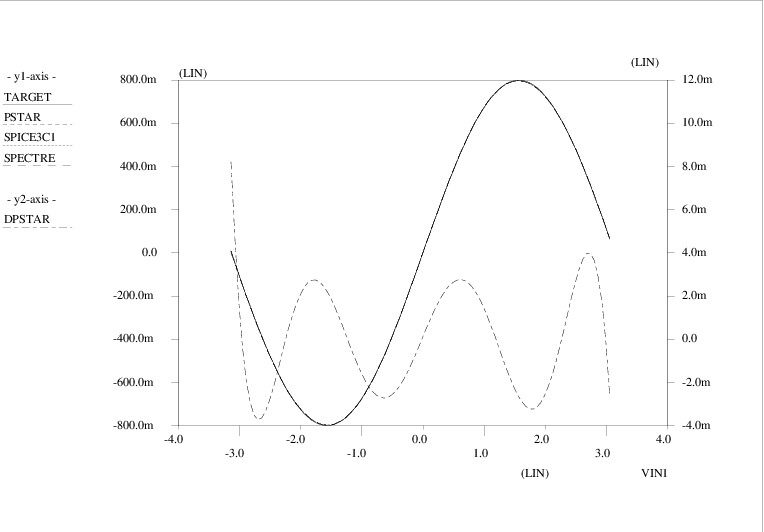
The Pstar model was then used in a Pstar run to simulate the model terminal current as a function of the branch voltage in the range [-π,π]. The SPICE model was similarly used in both Berkeley SPICE3c1 and Cadence Spectre. The results are shown in Fig. 4.5.

Figure 4.5:

Neural network mapped onto several circuit simulators.

The 3-neuron neural network simulation results of Pstar, SPICE3c1 and Spectre all nicely match the target data curve. The difference between Pstar outcomes and the target data is shown as a separate curve (“DPSTAR = PSTAR - TARGET”).

Of course, Pstar already has a built-in sine function and many other functions that can be used in defining controlled sources. However, the approach as outlined above would just as well apply to device characteristics for which no analytical expression is known, for instance by using curve traces coming directly from measurements. After all, the neural network modelling software did not “know” anything about the fact that a sine function had been used to generate the training data.

4.2.2 A Single-Neuron Neural Network Example

In this section, several aspects of time domain and frequency domain learning will be illustrated, by considering the training of a 1-1 neural network consisting of just a single neuron.

4.2.2.1 Illustration of Time Domain Learning

In Fig. 2.6, the step response corresponding to the left-hand side of the neuron differential equation (2.2) was shown, for several values of the quality factor Q. Now we will use the response as calculated for one particular value of Q, and use this as the target behaviour in a training set. The modelling software then adapts the parameters of a single-neuron neural network, until, hopefully, a good match is obtained. From the construction of the training set, we know in advance that a good match exists, but that does not guarantee that it will indeed be found through learning.

From a calculated response for τ_2,ik = 1 and Q = 4, the following corresponding training set was created, in accordance with the syntax as specified in Appendix B, and using 101 equidistant time points in the range t ∈ [0,25] (not all data is shown)

From Eq. (2.22) we find that the choices τ_2,ik = 1 and Q = 4 imply τ_1,ik = .

Figure 4.6:

Step response of a single-neuron neural network
as it adapts during subsequent learning iterations.

The neural modelling software was subsequently run for 25 Polak-Ribiere conjugate gradient iterations, with the option (s_ik) = s_ik set, and using trapezoidal time integration. The v-parameter was kept zero-valued during learning, since time differentiation of the network input is not needed in this case, but all other parameters were left free for adaptation. After the 25 iterations, τ₁ had obtained the value 0.237053, and τ₂ the value 0.958771, which corresponds to Q = 4.1306 according to Eq. (2.22). These results are already reasonably close to the exact values from which the training set had been derived. Learning progress is shown in Fig. 4.6. For each of the 25 conjugate gradient iterations, the intermediate network response is shown as a function of the i_s-th discrete time point, where the notation i_s (in Fig. 4.6 written as i_s) corresponds to the usage in Eq. (3.18).

The step response of the single-neuron neural network after the 25 learning iterations indeed closely approximates the step response for τ_2,ik = 1 and Q = 4 shown in Fig. 2.6.

4.2.2.2 Frequency Domain Learning and Model Generation

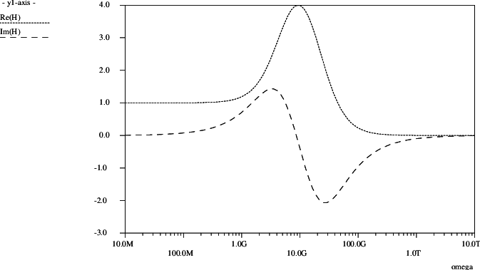
In Figs. 3.1 and 3.2, the ac behaviour was shown for a particular choice of parameters in a 1-1 network. One could ask whether a neural network can indeed learn this behaviour from a corresponding set of real and imaginary numbers. To test this, a training set was constructed, containing the complex-valued network transfer target values for a 100 frequency points in the range ω ∈ [10⁷,10¹³].

The input file snnn.n for the neural modelling software contained (not all data shown)

The frequency points are equidistant on a logarithmic scale. The neural modelling software was run for 75 Polak-Ribiere conjugate gradient iterations, with the option (s_ik) = s_ik set, and with a request for Pstar neural model generation after finishing the 75 iterations. The program started with random initial parameters for the neural network. An internal frequency scaling was (amongst other scalings) automatically applied to arrive at an equivalent problem and network in order to compress the value range of network parameters. Without such scaling measures, learning the values of the timing parameters would be very difficult, since they are many orders of magnitude smaller than most of the other parameters. In the generation of neural behavioural models, the required unscaling is automatically applied to return to the original physical representation. Shortly after 50 iterations, the modelling error was already zero, apart from numerical noise due to finite machine precision.

The automatically generated Pstar neural model description was

The Pstar neural network model name snnn0 is derived from the name of the input file with target data, supplemented with an integer to denote different network definitions in case several networks are trained in one run. Clearly, the modelling software had no problem discovering the correct values τ₁ = 2.5 ⋅ 10^-10s and τ₂ = 10^-20s², as can be seen from the argument list of NeuronType1_2(IN2,OUT2,REF). Due to the fact that we had a linear problem, and used a linear neural network, there is no unique solution for the remaining parameters. However, because the modelling error became (virtually) zero, this shows that the software had found an (almost) exact solution for these parameters as well.

Figure 4.7:

Fig. 3.1, 3.2 behaviour as recovered via the neural modelling software, automatic Pstar model generation, Pstar simulation and CGAP output.

The above Pstar model was used in a Pstar job that “replays” the inputs as given in the training set⁵. Fig. 4.7 shows the Pstar simulation results presented by the CGAP plotting package. This may be compared to the real and imaginary curves shown in Fig. 3.2.

4.2.3 MOSFET DC Current Modelling

A practical problem in demonstrating the potential of the neural modelling software for automatic modelling of highly nonlinear multidimensional dynamic systems, is that one cannot show every aspect in one view. The behaviour of such systems is simply too rich to be captured by a single plot, and the best we can do is to highlight each aspect in turn, as a kind of cross-section of a higher-dimensional space of possibilities. The preceding examples gave some impression about the nonlinear (sine) and the dynamic (non-quasistatic, time and frequency domain) aspects. Therefore, we will now combine the nonlinear with the multidimensional aspect, but for clarity only for (part of) the static behaviour, namely for the dc drain current of an n-channel MOSFET as a function of its terminal voltages.

Figure 4.8:

MOST model 901 dc drain current I_d(V _gd,V _gs).

Figure 4.9:

Neural network dc drain current I_d(V _gd,V _gs).

Figure 4.10:

Differences between MOST model 901 and neural network.

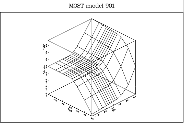
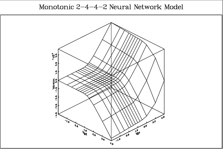
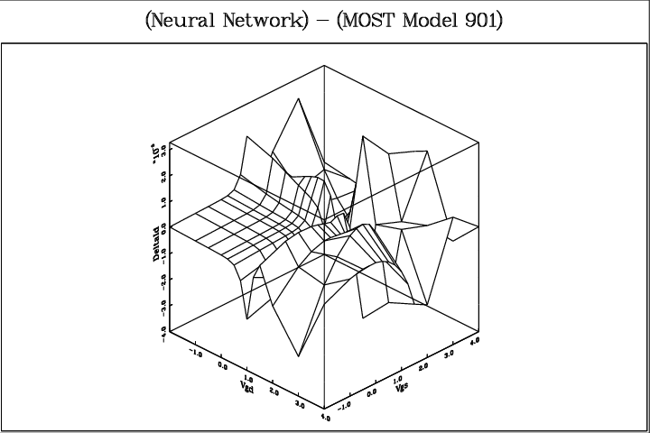
Fig. 4.8 shows the dc drain current I_d of the Philips’ MOST model 901 as a function of the gate-source voltage V _gs and the gate-drain voltage V _gd, for a realistic set of model parameters. The gate-bulk voltage V _gb was kept at a fixed 5.0V. MOST model 901 is one of the most sophisticated physics-based quasistatic MOSFET models for CAD applications, making it a reasonable exercise to use this model to generate target data for neural modelling⁶. The 169 drain current values of Fig. 4.8 were obtained from Pstar simulations of a single-transistor circuit, containing a voltage-driven MOST model 901. The 169 drain current values and 169 source current values resulting from the dc simulations subsequently formed the training set⁷ for the neural modelling software. A 2-4-4-2 network, as illustrated in Fig. 1.2, was used to model the I_d(V _gd,V _gs) and I_s(V _gd,V _gs) characteristics. The bulk current was not considered. During learning, the monotonicity option was active, resulting in dc characteristics that are, contrary to MOST model 901 itself, mathematically guaranteed to be monotonic in V _gd and V _gs. The error function used was the simple square of the difference between output current and target current—as used in Eq. (3.22). This implies that no attempt was made to accurately model subthreshold behaviour. When this is required, another error function can be used to improve subthreshold accuracy—at the expense of accuracy above threshold. It really depends on the application what kind of error measure is considered optimal. In an initial trial, 4000 Polak-Ribiere conjugate gradient iterations were allowed. The program started with random initial parameters for the neural network, and no user interaction or intervention was needed to arrive at behavioural models with the following results.

Fig. 4.9 shows the dc drain current according to the neural network, as obtained from Pstar simulations with the corresponding Pstar behavioural model⁸. The differences with the MOST model 901 outcomes are too small to be visible even when the plot is superimposed with the MOST model 901 plot. Therefore, Fig. 4.10 was created to show the remaining differences. The largest differences observed between the two models, measuring about 3 × 10^-5 A, are less than one percent of the current ranges of Figs. 4.8 and 4.9 (approx. 4 × 10^-3 A). Furthermore, monotonicity and infinite smoothness are guaranteed properties of the neural network, while the neural model was trained in 8.3 minutes on an HP9000/735 computer⁹.

This example concerns the modelling of one particular device. To include scaling effects of geometry and temperature, one could use a larger training set containing data for a variety of temperatures and geometries¹⁰, with additional neural network inputs for geometry and temperature. Alternatively, one could manually add a geometry and temperature scaling model to the neural model for a single device, although one then has to be extremely cautious about the different geometry scaling of, for instance, dc currents and capacitive currents as known from physical quasistatic modelling.

High-frequency non-quasistatic behaviour can in principle also be modelled by the neural networks, while MOST model 901 is restricted to quasistatic behaviour only. Until now, the need for non-quasistatic device modelling has been much stronger in high-frequency applications containing bipolar devices. Static neural networks have also been applied to the modelling of the dc currents of (submicron) MOSFETs at National Semiconductor Corporation [35]. A recent article on static neural networks for MOSFET modelling can be found in [43].

Figure 4.11:

MOSFET modelling error plotted logarithmically as a function of iteration count, using four independently trained neural networks.

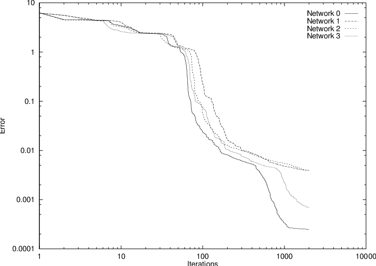
After the above initial trial, an additional experiment was performed, in which several neural networks were trained simultaneously. To give an impression about typical learning behaviour, Fig. 4.11 shows the decrease of modelling error with iteration count for a small population consisting of four neural networks, each having a 2-4-4-2 topology. The network parameters were randomly initialized, and 2000 Polak-Ribiere conjugate gradient iterations were allowed, using a sum-of-squares error measure—the contribution from Eq. (3.20) with Eq. (3.22).

Fig. 4.11 and Table 4.2 demonstrate that one does not need a particularly “lucky” initial parameter setting to arrive at satisfactory results.

4.2.4 Example of AC Circuit Macromodelling

For the neural modelling software, it does in principle not matter from what kind of system the training data was obtained. Data could have been sampled from an individual transistor, or from an entire (sub)circuit. In the latter case, when developing a model for (part of) the behaviour of a circuit or subcircuit, we speak of macromodelling, and the result of that activity is called a macromodel. The basic aim is to replace a very complicated description of a system—such as a circuit—by a much more simple description—a macromodel—while preserving the main relevant behavioural characteristics, i.e., input-output relations, of the original system.

Figure 4.12:

Amplifier circuit used in twoport analysis, and neural macromodel.

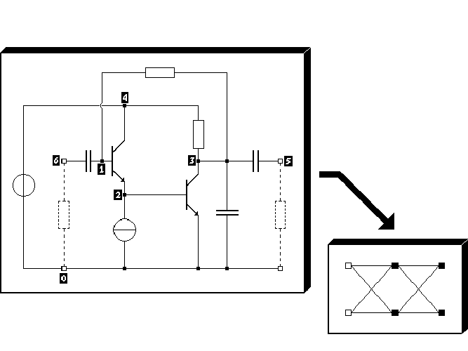
Here we will consider a simple amplifier circuit of which the corresponding circuit schematic is shown in Fig. 4.12. Source and load resistors are required in a Pstar twoport analysis, and these are therefore indicated by two dashed resistors. Admittance matrices Y of this circuit were obtained from the following Pstar job:

which generates textual output that has the numeric elements in the correct order for creating a training set according to the syntax as specified in Appendix B. In the above Pstar circuit definition block, each line contains a component name, separated from an occurrence indicator by an underscore, and followed by node numbers between parentheses and a parameter value or the name of a parameter list.

Figure 4.13:

(Y )₁₁ for amplifier circuit and neural macromodel. The circuit and neural model outcomes virtually coincide. IM(Y11CIRCUIT) and IM(Y11NEURAL) both approach zero at low frequencies.

Figure 4.14:

(Y )₂₁ for amplifier circuit and neural macromodel. The circuit and neural model outcomes virtually coincide. IM(Y21CIRCUIT) and IM(Y21NEURAL) both approach zero at low frequencies.

Figure 4.15:

(Y )₁₂ for amplifier circuit and neural macromodel. IM(Y12CIRCUIT) and IM(Y12NEURAL) both approach zero at low frequencies.

Figure 4.16:

(Y )₂₂ for amplifier circuit and neural macromodel. The circuit and neural model outcomes virtually coincide. IM(Y22CIRCUIT) and IM(Y22NEURAL) both approach zero at low frequencies.

The amplifier circuit contains two npn bipolar transistors, represented by Pstar level 1 models having three internal nodes, and a twoport is defined between input and output of the circuit, giving a 2 × 2 admittance matrix Y . The data resulting from the Pstar ac analysis were used as the training data for a single 2-2-2 neural network, hence using only four neurons. Two network inputs and two network outputs are needed to get a 2 × 2 neural network transfer matrix H that can be used to represent the admittance matrix Y . The nonnumeric strings in the Pstar monitor output are automatically neglected. For instance, in a Pstar output line like “MONITOR: REAL(Y21) = 65.99785E-03” only the substring “65.99785E-03” is recognized and processed by the neural modelling software, making it easy even to manually construct a training set by some cutting and pasting. A -trace option in the software can be used to check whether the numeric items are correctly interpreted during input processing. The neurons were all made linear, i.e., (s_ik) = s_ik, because bias dependence is not considered in a single Pstar twoport analysis. Only a regular sum-of-squares error measure—see Eqs. (3.61) and (3.62)—was used in the optimization. The allowed total number of iterations was 5000. During the first 500 iterations the before-mentioned heuristic optimization technique was used, followed by 4500 Polak-Ribiere conjugate gradient iterations.

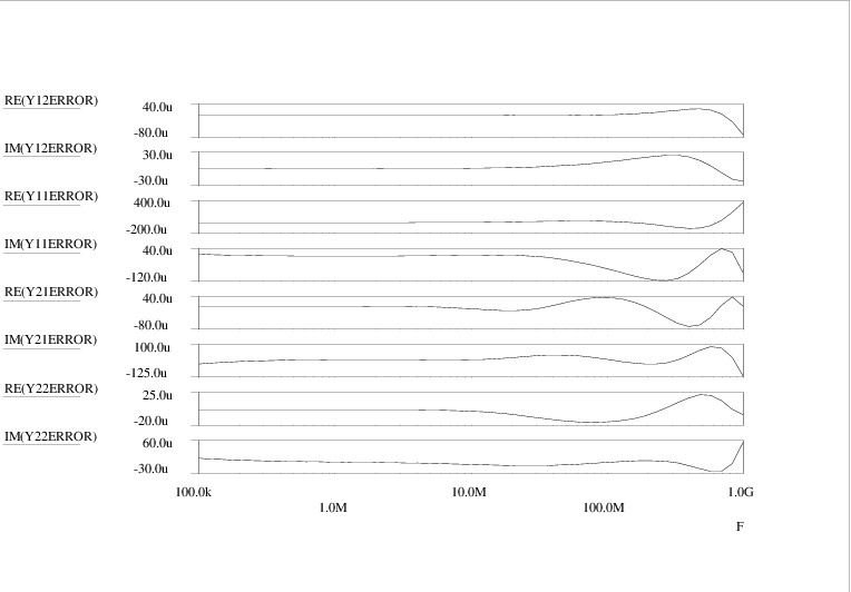
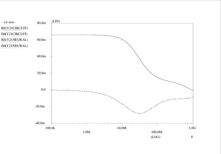
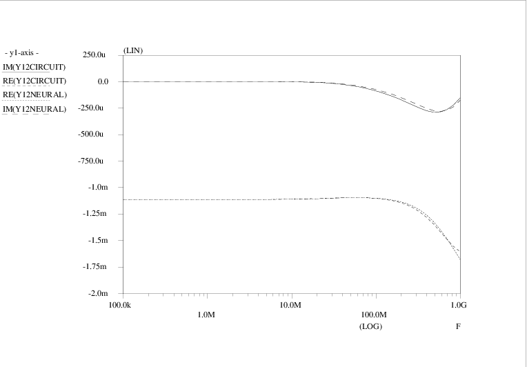
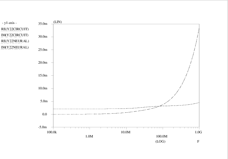
The four admittance matrix elements (Y )₁₁, (Y )₁₂, (Y )₂₁ and (Y )₂₂ are shown as a function of frequency in Figs. 4.13, 4.15, 4.14 and 4.16, respectively. Curves are shown for the original Pstar simulations of the amplifier circuit, constituting the target data Y<i><j>CIRCUIT, as well as for the Pstar simulations Y<i><j>NEURAL of the automatically generated neural network model in Pstar syntax. The curves for the imaginary parts IM(⋅) of admittance matrix elements are easily distinguished from those for the real parts RE(⋅) by noting that the imaginary parts vanish in the low frequency limit.

Apparently a very good match with the target data was obtained: for (Y )₁₁, (Y )₂₁ and (Y )₂₂, the deviation between the original circuit behaviour and the neural network behaviour is barely visible. Even (Y )₁₂ was accurately modelled, in spite of the fact that the sum-of-squares error measure gives relatively little weight to these comparatively small matrix elements.

Figure 4.17:

Overview of macromodelling errors as a function of frequency.

An overview of the modelling errors is shown in Fig. 4.17, where the error was defined as the difference between the neural network outcome and the target value, i.e., Y<i><j>ERROR = Y<i><j>NEURAL - Y<i><j>CIRCUIT.

4.2.5 Bipolar Transistor AC/DC Modelling

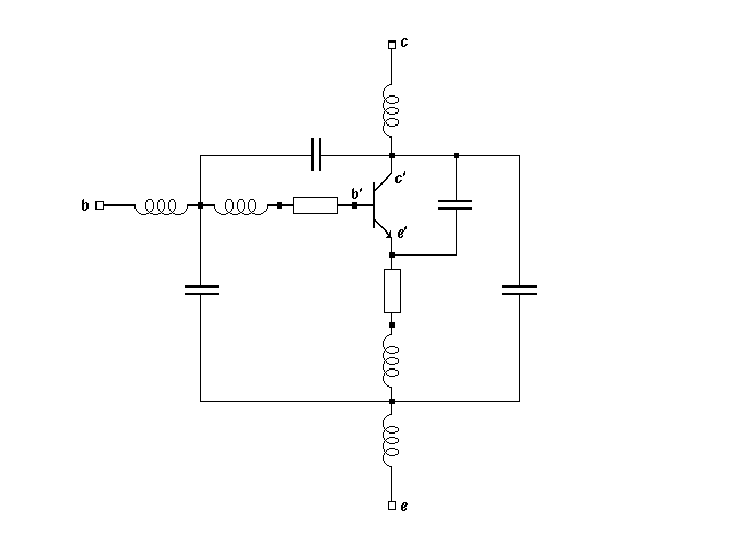
As another example, we will consider the modelling of the highly nonlinear and frequency-dependent behaviour of a packaged bipolar device. The experimental training values in the form of dc currents and admittance matrices for a number of bias conditions were obtained from Pstar simulations of a Philips model of a BFR92A npn device. This model consists of a nonlinear Gummel-Poon-like bipolar model and additional linear components to represent the effects of the package. The corresponding circuit is shown in Fig. 4.18.

Figure 4.18:

Equivalent circuit for packaged bipolar transistor.

Teaching a neural network to behave as the BFR92A turned out to require many optimization iterations. A number of reasons make the automatic modelling of packaged bipolar devices difficult:

• The linear components in the package model can lead to band-pass filter type peaks as well as to true resonance peaks that are “felt” by the modelling software even if these peaks lie outside the frequency range of the training data. The allowed quality factors of the neurons must be constrained to ensure that unrealistically narrow resonance peaks do not arise (temporarily) during learning; otherwise such peaks must subsequently be “unlearned” at significant computational expense.
• The dc currents are strongly dependent on the base-emitter voltage, and far less dependent on the collector-emitter voltage (Early effect), while the most relevant and rather narrow range of base-emitter voltages lies above 0.5V. An origin-shifting scaling is therefore required to ease the learning.
• The dc base currents are normally much smaller than the collector dc currents: that is what makes such a device useful. However, at high frequencies, the base and collector currents (both the real and imaginary parts) become much less different in size, due to the Miller effect. A network scaling based on dc data only may then be inappropriate, and lead to undesirable changes in the relative contributions of admittance matrix elements to the error measure.
• The position of extreme values in the admittance matrix elements as a function of frequency is bias dependent due to nonlinear effects.

This list could be continued, but the conclusion is that automatically modelling the rich behaviour of a packaged bipolar device is far from trivial.

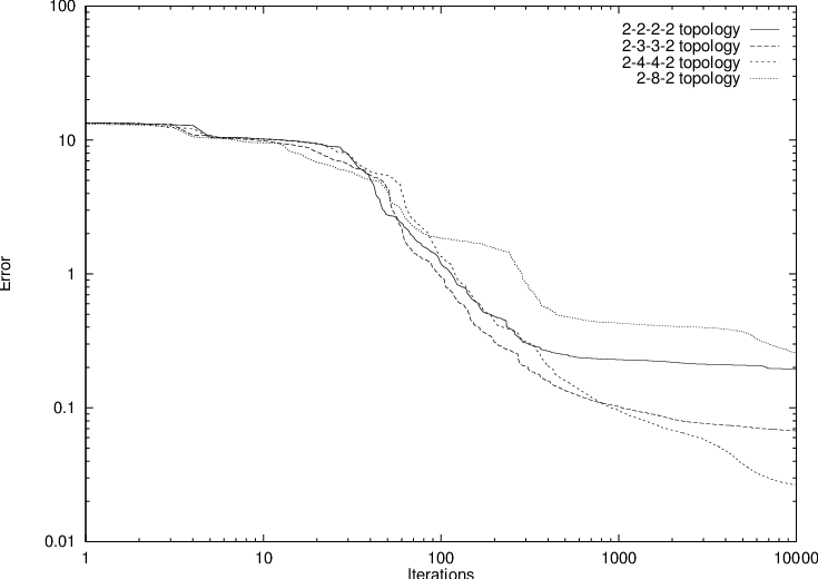
The (slow) learning observed with several neural network topologies is illustrated in Fig 4.19, using 10000 Polak-Ribiere conjugate gradient iterations. The DC part of the training data consisted of all 18 combinations of the base-emitter voltage V _be = 0, 0.4, 0.7, 0.75, 0.8 and 0.85 V with the collector-emitter voltage V _ce = 2, 5 and 10 V. The AC part consisted of 2 × 2 admittance matrices for 7 frequencies f = 1MHz, 10MHz, 100MHz, 200MHz, 500MHz, 1GHz and 2GHz, each at a subset of 8 of the above DC bias points:
(V _be,V _ce) = (0.8,2), (0,5), (0.75,5), (0.8,5), (0.85,5), (0.75,10), (0.8,10) and (0.85,10) V.

Figure 4.19:

Bipolar transistor modelling error plotted logarithmically as a function of iteration count.

The largest absolute errors in the terminal currents for the 18 DC points, as a percentage of the target current range (for each terminal separately), at the end of the 10000 iterations, are shown in Table 4.3.

Figure 4.20:

Neural network model with 2-4-4-2 topology compared to the bipolar discrete device model.

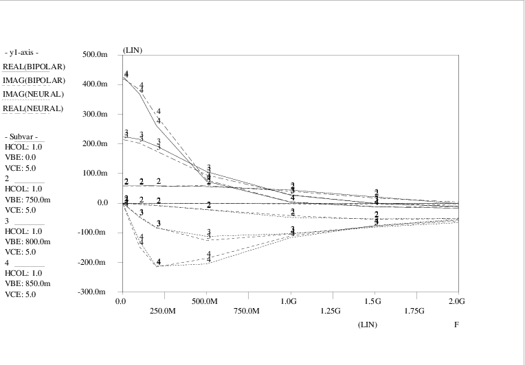
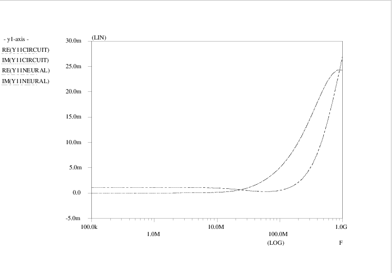
The 2-4-4-2 topology (illustrated in Fig. 1.2) here gave the smallest overall errors. Fig. 4.20 shows some Pstar simulation results with the original Philips model and an automatically generated behavioural model, corresponding to the 2-4-4-2 neural network. The curves represent the complex-valued collector current with an ac source between base and emitter, and for several base-emitter bias conditions. These curves show the bias- and frequency-dependence of the complex-valued bipolar transadmittance (of which the real part in the low-frequency limit is the familiar transconductance).

In spite of the slow learning, an important conclusion is that dynamic feedforward neural networks apparently can represent the behaviour of such a discrete bipolar device. Also, to avoid misunderstanding, it is important to point out that Fig. 4.20 shows only a small part (one out of four admittance matrix elements) of the behaviour in the training data: the learning task for modelling only the curves in Fig. 4.20 would have been much easier, as has appeared from several other experiments.

4.2.6 Video Circuit AC & Transient Macromodelling

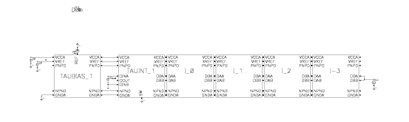
As a final example, we will consider the macromodelling of a video filter designed at Philips Semiconductors Nijmegen. The filter has two inputs and two outputs for which we would like to find a macromodel. The dynamic response to only one of the inputs was known to be relevant for this case. The nearly linear integrated circuit for this filter contains about a hundred bipolar transistors distributed over six blocks, as illustrated in Fig. 4.21. 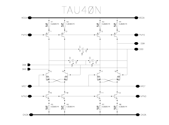The rightmost four TAUxxN blocks constitute filter circuits, each of them having a certain delay determined by internal capacitor values as selected by the designer. Fig. 4.22 shows the circuit schematic for a single 40ns filter section. The TAUINT block in the block diagram of Fig. 4.21 performs certain interfacing tasks that are not relevant to the macromodelling. Similarly, the dc biasing of the whole filter circuit is handled by the TAUBIAS block, but the functionality of this block need not be covered by the macromodel. From the circuit schematics in Fig. 4.24 and Fig. 4.25 it is clear that the possibility to neglect all this peripheral circuitry in macromodelling is likely to give by itself a significant reduction in the required computational complexity of the resulting models. Furthermore, it was known that each of the filter blocks behaves approximately as a second order linear filter. Knowing that a single neuron can exactly represent the behaviour of a second order linear filter, a reasonable choice for a neural network topology in the form of a chain of cascaded neurons would involve at least four non-input layers. 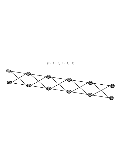We will use an extra layer to accommodate some of the parasitic high-frequency effects, using a 2-2-2-2-2-2 topology as shown in Fig. 4.23. The neural network will be made linear in view of the nearly linear filter circuit, thereby again gaining a reduction in computational complexity. The linearity implies (s_ik) = s_ik for all neurons. Although the video filter has separate input and output terminals, the modelling will for convenience be done as if it were a 3-terminal device in the interpretation of Fig. 2.1 of section 2.1.2, in order to make use of the presently available Pstar model generator¹¹.

Figure 4.21:

Block schematic of the entire video filter circuit.

Figure 4.22:

Schematic of one of the four video filter/delay sections.

Figure 4.23:

The 2-2-2-2-2-2 feedforward neural network used for macromodelling the video filter circuit.

The training set for the neural network consisted of a combination of time domain and frequency domain data. The entire circuit was first simulated with Pstar to obtain this data. A simulated time domain sweep running from 1MHz to 9.5MHz in 9.5μs was applied to obtain a time domain response sampled every 5ns, giving 1901 equidistant time points. In addition, admittance matrices were obtained from small signal AC analyses at 73 frequencies running from 110kHz to 100MHz, with the sample frequencies positioned almost equidistantly on a logarithmic frequency scale. Because only one input was considered relevant, it was more efficient to reduce the 2 × 2 admittance matrix to a 2 × 1 matrix rather than including arbitrary (e.g., constant zero) values in the full matrix.

Figure 4.24:

Schematic of the video filter interfacing circuitry.

Figure 4.25:

Schematic of the video filter biasing circuitry.

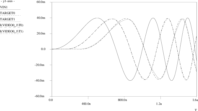
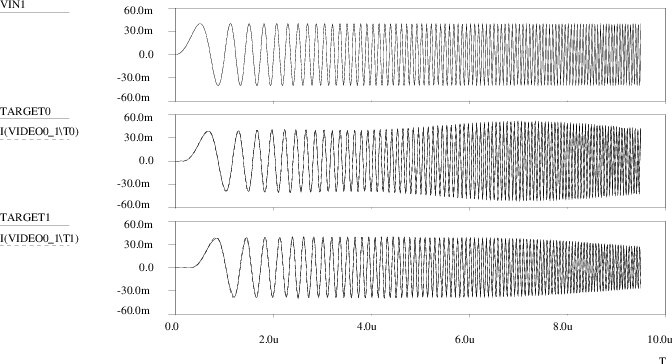
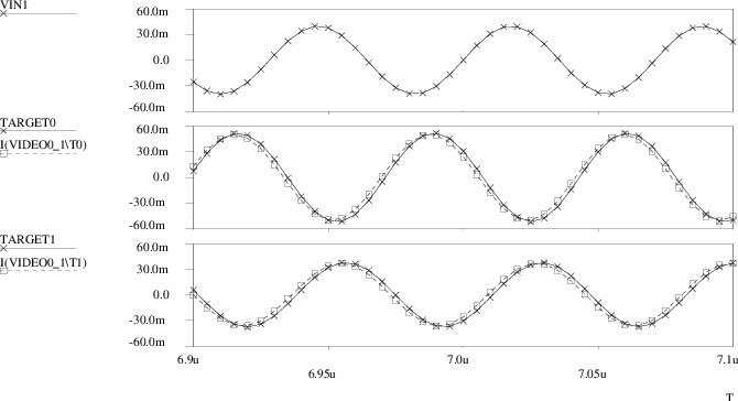
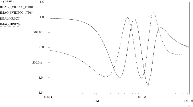
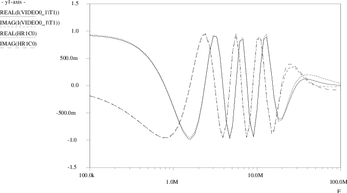
A comparison between the outcomes of the original transistor level simulations and the Pstar simulation results using the neural macromodel is presented in Figs. 4.26 through 4.30. In Fig. 4.26, VIN1 is the applied time domain sweep, while TARGET0 and TARGET1 represent the actual circuit behaviour as stored in the training set. The corresponding neural model outcomes are I(VIDEO0_1\T0) and I(VIDEO0_1\T1), respectively. Fig. 4.27 shows an enlargement for the first 1.6μs, Fig. 4.28 shows an enlargement around 7μs. One finds that the linear neural macromodel gives a good approximation of the transient response of the video filter circuit. Fig. 4.29 and Fig. 4.30 show the small-signal frequency domain response for the first and second filter output, respectively. The target values are labeled HR0C0 for H₀₀ and HR1C0 for H₁₀, while currents I(VIDEO0_1\T0) and I(VIDEO0_1\T1) here represent the complex-valued neural model transfer through the use of an ac input source of unity magnitude and zero phase. The curves for the imaginary parts IMAG(⋅) are those that approach zero at low frequencies, while, in this example, the curves for the real parts REAL(⋅) approach values close to one at low frequencies. From these figures, one observes that also in the frequency domain a good match exists between the neural model and the video filter circuit.

Figure 4.26:

Time domain plots of the input and the two outputs of the video filter circuit and for the neural macromodel.

Figure 4.27:

Enlargement of the first 1.6μs of Fig. 4.26.

Figure 4.28:

Enlargement of a small time interval from Fig. 4.26 around 7μs, with markers indicating the position of sample points.

Figure 4.29:

Frequency domain plots of the real and imaginary parts of the transfer (H)₀₀ for both the video filter circuit and the neural macromodel.

Figure 4.30:

Frequency domain plots of the real and imaginary parts of the transfer (H)₁₀ for both the video filter circuit and the neural macromodel.

In the case of macro-modelling, the usefulness of an accurate model is determined by the gain in simulation efficiency¹². In this example, it was found that the time domain sweep using the neural macromodel ran about 25 times faster than if the original transistor level circuit description was used, decreasing the original 4 minute simulation time to about 10 seconds. This is clearly a significant gain if the filter is to be used repeatedly as a standard building block, and it especially holds if the designer wants to simulate larger circuits in which this filter is just one of the basic building blocks. The advantage in simulation speed should of course be balanced against the one-time effort of arriving at a proper macromodel, which may easily take on the order of a few man days and several hours of CPU time before sufficient confidence about the model has been obtained.

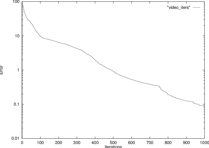
In this case, the 10-neuron model for the video filter was obtained in slightly less than an hour of learning time on an HP9000/735 computer, using a maximum quality factor constraint Q_max = 5 to discourage resonance peaks from occurring during the early learning phases. The results shown here were obtained through an initial phase using 750 iterations of the heuristic technique first mentioned in section 4.2 and outlined in section A.2, followed by 250 Polak-Ribiere conjugate gradient iterations¹³. The decrease of modelling error with iteration count is shown in Fig. 4.31, using a sum-of-squares error measure—the sum of the contributions from Eq. (3.20) with Eq. (3.22) and Eq. (3.61) with Eq. (3.62). The sudden bend after 750 iterations is the result of the transition from one optimization method to the next.

Figure 4.31:

Video filter modelling error plotted logarithmically as a function of iteration count.